(1)
where in (1) D stands for the specimen diameter and A for the intended spatial resolution.
Fig. 1
Standard µCT system components (source http://electroiq.com/blog/2011/03/3d-ct-x-ray-imaging-fills-inspection-gaps-says-xradia/)
As in standard CT imaging µCT is prone to a series of artifact. Image acquisition of biological tissue and metal implants generally suffers from so-called “Beam Hardening” [5, 7, 8]. This effect appears when materials with high density difference are imaged with a polychromatic X-ray source. In a polychromatic source the emitted photons have varying energy niveaus. Less energetic photons are easily absorbed in denser materials, while high energy photons travel through the materials. The emerging beam is “hardened” to consist only of high energy photons. If the beam passes a less dense material after hardening, the high energy photons are insignificantly absorbed, resulting in bad resolution along the path of the hardened beam. In images beam hardening results in “cupping”-artifacts such as “streaks” and “dark bands” (Fig. 2). A way to compensate this behaviour is to filter the beam before entering the specimen [8]. Standard filters against beam hardening are aluminium and copper and respectively, combinations of the two, with filter thicknesses between 0.2 and 1.0 mm [7, 8].
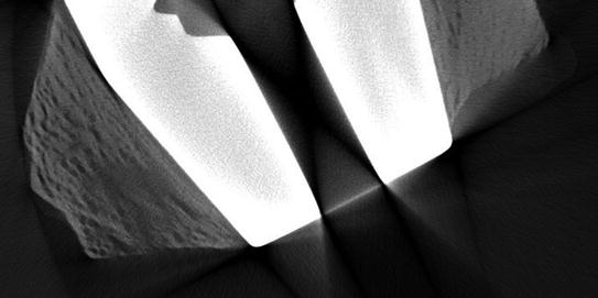
Fig. 2
Streaking artifacts (black lines) next to the edges of a titanium implant (white) integrated into a bone part
1.2 Osseointegration and Surface Properties
For sufficient durability and biocompatibility of weight-bearing bone implants the osseointegration is a determining factor. Initially introduced by Brânemark this concept described a procedure to measure the force fit of dental implants in jaw bone [1, 3]. Osseointegration generally describes the direct structural and functional connection between living bone tissue and surface of weight-bearing implant [9]. With growing implant specialization and therefore extending requirements for biocompatibility the measurement of osseointegration gains importance [3, 10, 11]. An implant is per definition osseointegrated when there is no progressive relative movement at the BII. Therefore, from the aspect of long-term compatibility osseointegration stands for an anchoring behavior of implants to be fully functional under system conditions (living tissue) without negative influence on biological reactions [11].
Information about osseointegration using histomorphometric analysis was only attainable by means of trabecular thickness, distance and number. This however, was only usable as a priori knowledge to describe the possible 3D tissue structure. Since the underlying algorithms are based on probabilistic models there is only limited qualitative and even less quantitative data gained from BII models from histomorphometry. The need for a 3D analysis standard is stated in various studies lead to the focus on imaging procedures an 3D tissue reconstruction algorithms and software [10, 12]. As a consequence the evaluation of the BII with modifiable implant surface parameters became an important research area. Customized surface coatings were developed which induce specific biological reactions to support or deny implant integration into tissue. This surface biocompatibility enables implant integration almost independently from the main implant material. The quantitative evaluation of the implant integration by 3D analysis of its BII is an important way to implant optimization and functionalization.
1.3 Medical Image Processing
The processing of clinically relevant medical images is mainly used in diagnose- and treatment-related tasks. In general image processing steps are applied to enhance the visualization of anatomical structures and to detect perceptible pathological symptoms.
Medical image processing technology comprises image registration, segmentation, analysis, pattern detection, 3D-visualization and virtual & augmented reality [13–15].
A crucial part of this study is the processing pipeline for 3D-visualization of medical imaging data (Fig. 3). Depending on the image quality the pipeline has a pre- and post- processing working around segmentation and reconstruction steps.
Fig. 3
Image processing pipeline steps
Image preprocessing is used to increase the image information and quality and directly dependent on the study requirements and image acquisition quality. Contents of this step are noise reduction, artifact reduction, contrast enhancement, scaling and resampling. These filtering operations are performed locally pixel- or voxel- wise with so-called “masks”. Masks are predefined fields of pixels to be processed on in one step. Depending on the filtering mask dimensions are specified with a “kernel size”, where a filtering mask with a kernel of 5 is comprised of a pixel field of 5 pixel height and width. Common filters are used to smooth the grey values of an image with each pixels receiving the mean grey value of all pixels in the specified mask.
1.4 Segmentation and 3D-Reconstruction
The segmentation process is used to label pixels with similar information content and group them in distinct classes of material. This step is used for classification purposes and for pattern recognition. The aim is to raise the image calculation from strictly pixel-related computations to symbol- and object-oriented processing [16, 17]. Segmentation methods range from point-oriented methods (global thresholding) over edge- and contour-oriented methods (random walker, snakes algorithm) to region-based methods (region growing). The global thresholding uses the information stored in the image histograms to separate pixel areas with the same gray value that can be quantitatively separated from each other. Every pixel that is above a certain gray value threshold is added to different segment then the ones below it. Subsequently, a surface reconstruction can be calculated on the separated pixel areas over all images in a µCT image stack. With algorithms like Marching-Cubes surfaces are generated over a finite number of voxels and their respective boundaries as defined in the segmentation process. With two adjacent segments it is possible to calculate the intersecting surface area of these segments with each other.
2 Methods and Material
Sample implants made of TiAlV were coated with plasma-polymerized ethylenediamine (PPEDA) and plasma-polymerized allylamine (PPAAm) and compared with a non-coated control group regarding bone-implant-interface area (BIIA) (Fig. 4). For each polymer coating and the non-coated group six specimens were implanted into distal rat femur. After 5 weeks specimens were removed and image data was acquired individually with a µCT-Setup.
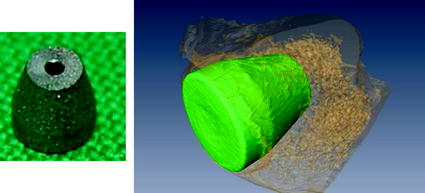
Fig. 4
Titanium implant (left), reconstructed surface models of implant (green) and surrounding bone (orange) (right) (Color figure online)
2.1 Image Data Acquisition and Preprocessing
Image data of the specimen were acquired individually with a micro-computer-tomograph (μCT) Nanotom 180nF (phoenix nanotom®, GE Measurement and Control solutions, phoenix|x-ray, Germany). A molybdenum target was used for X-ray beam generation. Voltage and current were set to 70 kV and 135 μA, to reach the optimum contrast. The μCT X-ray source used a cone-beam with vertical specimen alignment. The samples rotated 360° in 0.75° steps. Each step included three 2D images resulting in 1440 2D acquired images for one sample. The region-of-interest (ROI) for the 2D images was set in the range of the implant surface with approximately 1 mm surrounding bone tissue. Due to anatomical differences of the tibiae, the distance of the samples to the X-ray-tube and the detector, consequently varying the magnification and voxel size. Each specimen 2D data records included 7 GB of data volume and were used for generation of the 3D volume of the sample. The reconstruction of CT data (composing X-ray 2D images to a 3D volume) was performed with datos|x-reconstruction (GE, Germany). Titanium implants are harder to penetrate by X-rays in comparison to bone. Therefore, a beam-hardening correction of 6.7 was used to compensate for the inhomogeneous reconstructed volume of the implant and reach similar grey values inside the entire implant. For further processing, the transformation of the volume data in the DICOM data was required. Due to limited RAM capacity of the PC working station the data volume of each set had to be resampled to reduce the amount of processed data. Datasets were resampled with a Box-filter (2 × 2 × 2-kernel) reducing data volume by factor 8 and voxel resolution by factor 2 while preserving spatial voxel proportions. Subsequently datasets were filtered with an Unsharp-Masking algorithm (x-y-planes, 5×-kernels, Sharpness 0.6) to improve image quality for the following segmentation process. Additionally datasets were cropped to reduce data volume and approximate the volume of interest (VOI).
Related posts:
 Fusion for Computer-Assisted Bone Tumor Surgery
Three-Dimensional Imaging in Fracture Treatment with a Mobile C-Arm
Planning of Periacetabular Osteotomy (PAO)
Robotics for Musculoskeletal Surgery
of the Art of Ultrasound-Based Registration in Computer Assisted Orthopedic Interventions
Reconstruction-Based Planning of Total Hip Arthroplasty
Fusion for Computer-Assisted Bone Tumor Surgery
Three-Dimensional Imaging in Fracture Treatment with a Mobile C-Arm
Planning of Periacetabular Osteotomy (PAO)
Robotics for Musculoskeletal Surgery
of the Art of Ultrasound-Based Registration in Computer Assisted Orthopedic Interventions
Reconstruction-Based Planning of Total Hip Arthroplasty
Stay updated, free articles. Join our Telegram channel

Full access? Get Clinical Tree


