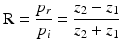
Fig. 1
Typical example of involved components in an ultrasound-based surgical navigation system: B-mode ultrasound probe, infrared tracking camera (=navigator), surgical tool (here: impactor), the therapeutic object (here: pelvis) to be operated and the virtual object (representation on a computer screen)
In the next section, the basic principles of ultrasound imaging will be explained, before ultrasound-based registration methods will be presented in detail. This chapter concludes with a summary on the clinical state of the art and an outlook on the future work of making ultrasound-based registration a valid alternative to pointer-based registration methods.
2 Basic Principles of Ultrasound Imaging
This section deals with the principles of ultrasound image formation and the basic physical concepts, which are relevant for the application of ultrasound imaging for intraoperative registration. An explanation of the basic principles is of particular importance for the understanding of the section on ultrasound-based registration algorithms.
Ultrasound is generally referring to a high-energy acoustic sound wave. Due to its high frequency, ultrasound waves can propagate within a matter medium and thus are extremely suitable to penetrate body tissue. Ultrasound waves, which are sent into an inhomogeneous medium such as the human body, are reflected and scattered at the boundaries of different tissue types. These reflections can be measured in terms of echoes. In medical ultrasound, these echoes are utilized to visualize inner structures of the human body. Typically used ultrasound frequencies for medical purpose are in the range of 2–30 MHz. An ultrasonic transducer (probe) is placed in direct contact to the skin or organ and short ultrasound pulses are continuously sent into the body. These pulses are accordingly reflected back towards the transducer at the different tissue boundaries and detected as echoes. By means of the time it takes for the echoes to return back to the transducer, the depth of these originating reflections can be determined.
Ultrasonic imaging can be operated in different modes. Depending on the medical purpose, various imaging modes exist. The simplest mode is the A-mode (amplitude mode). A single transducer element sends pulses of ultrasound waves and records the returning echo intensity (amplitude). Because only a single scan line exists, the resulting echoes are plotted as a curve in terms of the travel time. The travel time is directly related to the depth of the recorded echo and thus the A-mode is primarily used to measure the distance to certain structures. The most commonly used mode in the clinical routine is the B-mode (brightness mode). An array of transducer elements sends and receives ultrasound pulses and therefore represents an extension of the A-mode. As many transducer elements are simultaneously measuring the echo intensities, a cross-sectional image can be formed. Thereby, the pixel grayscale (brightness) of such a two-dimensional (2D) ultrasound image reflect the measured echo amplitude. Beside the commonly used A- and B-mode, Doppler ultrasonography and M-mode are frequently used in medical diagnostics. While the Doppler mode is particularly relevant to measure and visualize the blood flow, the M-mode (motion mode) is mainly used to determine the motion of organs such as the one of the heart. But mainly relevant for the intraoperative registration of bony structures are the A- and B-mode. While the A-mode can be used to measure the distance through the skin to a bony structure in a single direction, the B-mode is able to form a cross-sectional image and thus gives two-dimensional information of the anatomy treated with ultrasound.
While different A-mode transducer mainly differ in size, B-mode transducer differ in shape and size. Mainly relevant for the imaging of the musculoskeletal system is the linear array transducer. This transducer consists of a large number of linearly arranged elements and consequently generates a rectangular 2D ultrasound image. As conventional ultrasound imaging only provides two-dimensional information, two technologies can be used to retrieve 3D volumetric data. The first technology extends the B-mode imaging by attaching a trackable sensor (e.g. infrared light reflecting spheres) to the ultrasound transducer. It requires a tracking system, which measures the position and orientation of the trackable sensor in space. Thus, for each B-mode ultrasound image, a unique 3D transformation in space is recorded. As the transducer can be freely moved over the patient’s anatomy, this technique is referred to as “3D free-hand”. The second technique is based on a special 3D transducer and does not require a tracking system. This 3D transducer is able to sample a pyramidal volume by internally rotating the transducer array of up to 90°. As the acquisition angle of each single ultrasound image is internally encoded, the imaged 3D volume can be consequently assembled. For a detailed description of the functionality of such a 3D transducer I would like to refer to Hoskins et al. [29]. As the dimensions of the assembled image volume are restricted by the hardware, stitching techniques were developed to overcome this limitation [17, 52, 64]. But since the 3D free-hand technique allows for a more flexible image acquisition (volumes do not need to overlap), this technique is preferred over using a 3D transducer for ultrasound-based registration.
In order to correctly interpret a two-dimensional ultrasound image, it is important to understand the process of echo generation. As already indicated, echoes are generated when the ultrasound waves encounter a change in the medium properties (e.g. at tissue boundaries). The relevant material properties are the medium density ρ and the stiffness k, which are expressed as the acoustic impedance z:

Generally speaking, the acoustic impedance describes the response of a medium to an incoming ultrasound wave of certain pressure p. The medium density and stiffness are also essential for the propagating speed c of the ultrasound waves:

Thus, the speed of sound is a material property and has been measured for all relevant tissue types of the human body. The speeds of sound for different tissue types are listed in Table 1. At a tissue boundary, the ultrasound wave is partially transmitted or reflected—depending on the involved acoustic impedances. This relationship can be expressed by the reflection coefficient R:
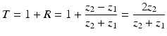
whereas p i and p r are the pressures of the incident and the reflected ultrasound waves. The ultrasound wave is thereby travelling from the first medium with acoustic impedance z 1 into the second medium with acoustic impedance z 2. Consequently, a transition between tissue types of similar acoustic impedance (z 1 ≈ z 2) will lead to a rather weak echo, while a transition between tissue types of great difference (e.g. z 2 ≫ z 1) in acoustic impedance will result in a strong echo. Out of the reflection coefficient, the transmission coefficient T can be determined. As the pressure in the first medium and the second medium must be the same (see Fig. 2), the pressure of the incident wave and of the reflecting wave equals to the one of the transmitted wave p t ,

Thereby the direction of the reflected wave is in the opposite direction to the incident wave. Out of this relationship, the transmission coefficient can be calculated as follows:
Out of the acoustic impedances of the first and the second medium, the amount of reflection and transmission can be calculated. The acoustic impedances for different tissue types are listed in Table 1.
(1)
(2)
(3)
(4)
(5)
Body tissue | Speed of sound c (m/s) | Acoustic impedance Z (Pa m−3 s) |
|---|---|---|
Fat | 1475 | 1.38 × 10⁶ |
Water | 1480 | 1.5 × 10⁶ |
Blood | 1570 | 1.61 × 10⁶ |
Muscle | 1580 | 1.70 × 10⁶ |
Bone | 3190–3406 | 6.47 × 10⁶ |
Average tissue | 1540 | 1.63 × 10⁶ |
Air | 333 | 0.00004 × 10⁶ |
Fig. 2
The incident wave is transmitted and reflected at the transition of the first and the second medium
Since the described reflection process is generally applicable to smooth interfaces, it is referred to as specular reflection. This type of reflection is important for the interpretation of the ultrasound image. In diffuse reflection, the ultrasound wave is reflected uniformly in all directions. It also largely contributes to the image formation, as it generates echoes from surfaces, which are not perpendicular to the ultrasound beam. A similar effect degrading the image quality is speckle noise. When a wave strikes particles of much smaller size compared to the ultrasound wavelength, echoes are scattered randomly in many directions. This speckle pattern is normally less bright than specular reflection and is frequently observed in ultrasound images of the liver and lung [11]. As it is not directly related to anatomical information, speckle noise is considered to be an ultrasound artifact. Another important ultrasound artifact is related to the assumption of a constant propagation of sound. As the ultrasound system assumes a value for speed of sound of 1540 m/s (corresponds to the average speed of sound in human soft tissue), echoes of tissues with deviating speed of sound (see Table 1) appear at an incorrect depth. This artifact might also degrade the ultrasound-based registration accuracy: A certain thick layer of fat d fat on top of the bone will lead to an echo delay (cfat < cavg) so that the depth of the bone surface would be displaced to a greater depth. The greater the penetration depth d tissue , the larger is the depth localization error. We will come back to this issue in the section on the ultrasound-based registration strategies.
3 Ultrasound-Based Registration
As indicated in the previous section, mostly relevant for the intraoperative registration step are A- and B-mode ultrasound imaging. Thus, this section focuses on the review of ultrasound-based registration techniques using A- or B-mode imaging published in the literature. While most of the presented methods are dealing with the registration of bones, some approaches are beyond orthopedics, but might get relevant for this field in the near future.
3.1 Registration Methods Using A-Mode Imaging
The direct replacement of pointer-based palpation by the acquisition of A-mode signals is quite evident. While the pointer-based digitization delivers a single 3D point at a time, A-mode imaging provides a one-dimensional signal in beam direction. Most commonly, this signal is processed using the Hilbert transform to determine the echo location related to the reflection of the wave from the bone surface [27, 42]. This however presumes that the beam axis of the A-mode transducer can be arranged perpendicular to the surface of the bone. In order to utilize a tracked A-mode transducer, a calibration step needs to be performed to relate the signal echo to a 3D point. Thus, the origin and the main axis of the ultrasound beam need to be determined with respect to the attached trackable sensor. As the case of the ultrasound transducer is normally of cylindrical shape, the symmetry axis of the case corresponds to the beam propagation axis. Therefore, the origin of the transducer and another point on the symmetry axis could be simply digitized with a tracked pointer to define the calibration parameters. A more advanced calibration method was presented by Maurer et al. [42]. They developed an ultrasound-based registration for the skull. A similar method was also presented by Amstutz et al. [3]. Both approaches used A-mode imaging to match the surface model derived from a CT-scan to the intraoperative situation. In a plastic bone study Maurer et al. [42] acquired 150 points to achieve a surface residual error of 0.20 mm. In addition, one patient trial was performed, obtaining a surface residual error of 0.17 mm for a set of 30 points. Sets of only 12–20 points were recorded by Amstutz et al. [3] in 12 patient trials, obtaining a mean surface registration error of 0.49 ± 0.20 mm. In order to overcome the difficulty of accurately aligning the A-mode transducer with respect to the bone surface, a man/machine interface was proposed by Heger et al. [27]. Instead of using an optical or magnetic tracking system, they proposed to use a mechanical localizer system. After an initial interactive registration step, the orientation of the transducer is adjusted, to get an optimal perpendicular alignment of the beam axis with respect to the bone surface. The approach was validated by repetitive registration of a femoral bone model, resulting in a mean root-mean-square (RMS) error of 0.59 mm. Similarly, A-mode registration of the pelvis was investigated by Oszwald et al. [49]. The surface matching accuracy was analyzed in an in vitro study using two synthetic pelvis models. The identified registration errors were in the range of 0.98–1.51 mm.
3.2 Registration Methods Using B-Mode Imaging
Even though, all presented approaches using A-mode ultrasound imaging for intraoperative registration showed promising results, its general application is restricted. A-mode imaging only allows the recording of single points at a time. As the angle of the beam axis to the bone surface has to be approximately 90°, the transducer cannot be easily swept over the area of interest. On the contrary, B-mode ultrasound allows a much more flexible image acquisition. Thus, the existing methods for B-mode ultrasound-based registration will be covered in greater detail.
3.2.1 B-Mode Calibration
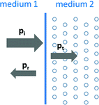
As indicated in the previous section, 3D free-hand B-mode imaging requires the attachment of a trackable sensor to the transducer. Consequently, a calibration step needs to be performed to relate 2D image information (in pixels) to the tracked 3D space (in mm). Figure 3 gives in overview on the involved coordinate systems and transformations.
Fig. 3
Overview on different coordinate-systems (in curly brackets) involved during an ultrasound-based registration
While the transformations of the patient {Pat} and the ultrasound transducer {US} are inherently known by the tracking system, the relationship between the tracked transducer coordinate-system {US} and the image coordinate-system  needs to be determined in a calibration step:
 is a scaling matrix and describes the transformation between the local 2D image coordinate-system
  and the 3D global image coordinate-system
  (see Fig. 3),
  is the transformation from the 3D global image coordinate-system
  to the 3D coordinate-system of the US probe {US} and
  is the resulting calibration transformation. This calibration transformation can be applied to transform 2D points in the ultrasound image
  to 3D points in the coordinate-system of the ultrasound transducer
  :
:
These 3D points can be further transformed to a point cloud  in common 3D patient space via the transformations of the trackable patient sensor
  and the ultrasound transducer
  with respect to the tracking camera:
The calibration transformation  consists of nine parameters: While
  contains the two mm-to-pixel scaling factors in x- and y-direction and a translation,
  has three degrees of freedom for translation and three for rotation. In order to determine these calibration parameters the general concept of image calibration is employed. Therefore, a calibration phantom of known geometrical properties is imaged and its features are detected on the ultrasound image. As the positions of the phantom features are known in physical space, the spatial relationship to its imaged features can be estimated using a least-squares approach. A comprehensive review of existing B-mode calibration techniques was presented by Mercier et al. [43]. According to this review, all calibration phantoms have a common setup: They consist either of small spherical objects or of intersecting wires and are placed in a container of a coupling medium. During the calibration procedure, the probe is adjusted to image all relevant phantom features. The features are either automatically or interactively segmented on the image and used to find the unknown calibration parameters [43]. Even though, ultrasound calibration is a standard procedure, it is actually only valid for a specific speed of sound. Thus, most commonly water is used as its speed of sound corresponds to the one of the average speed of sound of soft tissue (1540 m/s). But for a medium with a speed of sound different than the one used for calibration, a depth localization error will occur. While the translational and rotational parameters of
  purely rely on the hardware configuration (see Fig. 3), only the scaling factor in scanning direction of
  is affected by a deviating speed of sound. Techniques to compensate for this deficiency will be presented later in this section.
needs to be determined in a calibration step:(6)
is a scaling matrix and describes the transformation between the local 2D image coordinate-system and the 3D global image coordinate-system (see Fig. 3), is the transformation from the 3D global image coordinate-system to the 3D coordinate-system of the US probe {US} and is the resulting calibration transformation. This calibration transformation can be applied to transform 2D points in the ultrasound image to 3D points in the coordinate-system of the ultrasound transducer :(7)
in common 3D patient space via the transformations of the trackable patient sensor and the ultrasound transducer with respect to the tracking camera:(8)
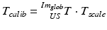
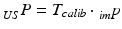
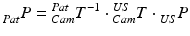
consists of nine parameters: While contains the two mm-to-pixel scaling factors in x- and y-direction and a translation, has three degrees of freedom for translation and three for rotation. In order to determine these calibration parameters the general concept of image calibration is employed. Therefore, a calibration phantom of known geometrical properties is imaged and its features are detected on the ultrasound image. As the positions of the phantom features are known in physical space, the spatial relationship to its imaged features can be estimated using a least-squares approach. A comprehensive review of existing B-mode calibration techniques was presented by Mercier et al. [43]. According to this review, all calibration phantoms have a common setup: They consist either of small spherical objects or of intersecting wires and are placed in a container of a coupling medium. During the calibration procedure, the probe is adjusted to image all relevant phantom features. The features are either automatically or interactively segmented on the image and used to find the unknown calibration parameters [43]. Even though, ultrasound calibration is a standard procedure, it is actually only valid for a specific speed of sound. Thus, most commonly water is used as its speed of sound corresponds to the one of the average speed of sound of soft tissue (1540 m/s). But for a medium with a speed of sound different than the one used for calibration, a depth localization error will occur. While the translational and rotational parameters of purely rely on the hardware configuration (see Fig. 3), only the scaling factor in scanning direction of is affected by a deviating speed of sound. Techniques to compensate for this deficiency will be presented later in this section.The main goal of ultrasound-based registration is the fusion of a preoperative planning with the intraoperative situation. Many different approaches have been published in literature. For convenience the existing approaches have been categorized according to their employed strategy. Accordingly, three main categories were determined:
landmark digitization
surface-based registration
volume-based registration
3.2.2 Landmark Digitization
Equivalent to the approaches using A-mode imaging, B-mode images could be used to digitize single bony landmarks. But instead of computing a registration transformation to preoperative image data, the digitized bony landmarks could be used to set up an intraoperative reference plane for safe implantation of acetabular cup implants [34, 50, 65]. This reference plane was employed by Jaramaz et al. [31] to guide the cup implantation during navigated total hip replacement. This plane—generally referred to as ‘anterior pelvic plane’ (APP)—requires the digitization of three pelvic landmarks and has been introduced by Lewinnek et al. [39]. They have investigated the relationship between the orientation of cup implants with respect to this APP and the probability of dislocation. They identified a ‘safe zone’, in which the dislocation rate was significantly low. As the cup orientation can be measured with respect to this APP in terms of two angles (anteversion and inclination), this safe zone defined the safe range for both angles. Thus, the common goal of a navigated total hip replacement is to place the cup implant within this safe zone. While conventionally, the corresponding APP landmarks were percutaneously digitized using a tracked pointer tool, some approaches proposed the use of B-mode imaging. Parratte et al. [50] compared the effect of percutaneous and ultrasound digitization of the APP landmarks. In an in vitro study, landmarks on two cadaveric specimen were digitized with both modalities. Higher reliability was found for the ultrasound modality. The same objective was investigated by Kiefer and Othman [34]. Comparing the data of 37 patient trials showed higher validity for the APP defined with ultrasound. Wassilew et al. [65] analyzed the accuracy of ultrasound digitization in a cadaver trial. In order to determine the ground truth APP, radio-opaque markers were placed into the cadaveric specimen before CT acquisition. The ground truth APP was defined in the CT-scan and transferred to the tracking space by locating the radio-opaque markers with a tracked pointer. Five observers repeated the ultrasound digitization five times for both cadaveric specimen, resulting in average errors for inclination of −0.1 ± 1.0° and for anteversion of −0.4 ± 2.7°.
While the first category dealt with the landmark digitization for setting up a reference system, the next two categories deal with the registration of intraoperative ultrasound data to preoperative images or statistical shape models (SSM) for extrapolating the sparse information. An overview of the individual components and their particular transformations is shown in Fig. 4. Thus, the primary goal of the all the methods being presented is to determine the transformation between the virtual data (e.g. CT, SSM) and the patient.
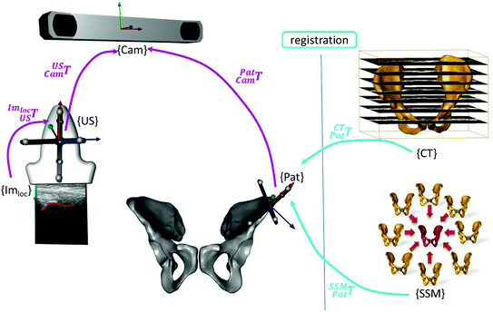
Fig. 4
Involved transformations during the image-guided intervention. The transformations highlighted in magenta color are either known by the trackable sensors  or due to the calibration step
  . The registration transformation in cyan color (e.g.
 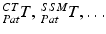 ) needs to be determined in a registration step. {US}, {Pat} and {Cam} represent the coordinate systems of the ultrasound probe, the patient and the tracking camera
or due to the calibration step . The registration transformation in cyan color (e.g. ) needs to be determined in a registration step. {US}, {Pat} and {Cam} represent the coordinate systems of the ultrasound probe, the patient and the tracking camera3.2.3 Surface Based Registration
For most surgical interventions the digitization of three landmarks is not sufficient to set up a reference system or to provide a valuable guidance to the surgeon. Particularly if preoperative image data and planning need to be visualized intraoperatively, a sophisticated method is required. A convenient approach is based on a registration of point clouds extracted from ultrasound images to a surface model. While the surface model could be segmented from the image data (e.g. from CT or MRI) prior to the surgery, the extraction of the point data from the ultrasound images followed by the actual registration step would need to take place on-line during the surgery. Thus, the first step to be solved is the segmentation of the ultrasound images. So far, many segmentation approaches have been published in literature. As most of them have been developed for a specific clinical application, I would like to highlight a few approaches with a focus on orthopedic applications. Thomas et al. [62] developed an automatic ultrasound segmentation method for estimating the femur length in fetal ultrasound images. They applied basic image processing algorithms such as morphological operators, contrast enhancement and thresholding to determine the bone surface. The method was validated by means of 24 ultrasound datasets, showing a good agreement to the manual measurement. An automatic segmentation based on a priori knowledge about the osseous interface and ultrasound physics was proposed by Daanen et al. [16]. This a priori knowledge was fused by the use of fuzzy logic to produce an accurate delineation of the sacrum. An extensive validation study with about 300 ultrasound images of cadavers and patients was conducted, showing a mean error of less than 1 mm. A more general segmentation approach was presented by Kowal et al. [36]. The first out of two steps determines a region of interest, which most likely contains the bone contour, while the second step tries to extract the bone contour. Both steps were based on general image processing algorithms and were tested with animal cadavers. A more sophisticated segmentation approach was proposed by Hacihaliloglu et al. [24]. They developed a special detector to extract ridge-like features for bone surface location using a 3D ultrasound probe. The work was further improved [26] and applied in a clinical study to support the imaging of distal radius fractures and pelvic ring injuries. On average, a surface fitting error of 0.62 ± 0.42 mm for pelvic patients and 0.21 ± 0.14 mm for distal radius patients was obtained. For more information on ultrasound segmentation I would like to refer to Noble and Boukerroui [46]. They conducted a very detailed survey on ultrasound segmentation, focusing their review only on papers with a substantial clinical validation.
Ionescu et al. [30] published one of the first approaches for the registration of ultrasound images to a segmented CT-scan. The ultrasound images were automatically segmented and rigidly matched to the surface model extracted from CT. The method was developed to intraoperatively guide the surgeon for inserting screws into the pedicle of vertebral bodies or into the sacro-iliac joint. In an in vitro study, the accuracy of the method was analyzed by means of a plastic spine model and a cadaveric pelvis specimen. Maximum errors of about 2 mm and 2° were found for both applications. A similar approach was proposed by Tonetti et al. [63] for iliosacral screwing. The ultrasound images were manually segmented and a surface-based registration algorithm was applied to determine the transformation to the preoperative CT-scan. The accuracy was analyzed by comparing it to the standard procedure of percutaneous iliosacral screwing using a fluoroscope. Thereby, the ultrasound-based technique showed higher precision and a lower complication rate. Amin et al. [1] combined the steps of ultrasound segmentation and CT registration for image-guided total hip replacement. After an initial landmark-based matching between the segmented CT-model and the intraoperative space, the aligned surface model of the pelvis is used as a shape prior to guide the ultrasound image segmentation. Thus, ultrasound segmentation and registration steps are solved simultaneously. The validity of the proposed approach was analyzed by means of a pelvic phantom model resulting in an average translational error of less than 0.5 mm and an average rotational error of less than 0.5°. In addition, 100 ultrasound images were recorded during a navigated surgery. In ten registration trials using a subset of 30 images each, the ultrasound-based registration was compared to conventional percutaneous pointer-based registration. A maximum difference of 2.07 mm in translation and of 1.58° in rotation was found. Barratt et al. [8] proposed a registration method to solve the error introduced by the assumption of a constant speed of sound. During the rigid registration between the ultrasound-derived points and the CT-segmented surface model not only the 3D transformation, but also the calibration matrix  is optimized. Therefore, the scaling in scanning direction (see Sect. 5.1) is included as a parameter in the optimization of the registration transformation. The accuracy was evaluated by the acquisition of ultrasound images of the femur and pelvis from three cadaveric specimen. Thereby, the ultrasound images were manually segmented and applied for the CT-based registration, yielding an average target registration error of 1.6 mm. A different clinical application of ultrasound to surface registration was presented by Beek et al. [9]. They developed a system to navigate the treatment of non-displaced scaphoid fractures. The trajectory of the screw to fix the fracture is planned using a CT-scan of the wrist joint and matched to the intraoperative scenario using ultrasound imaging. The accuracy of guided hole drilling was investigated in an in vitro study using 57 plastic bones and compared with conventional fluoroscopic guidance. On average, the surgical requirements were met and the accuracy of fluoroscopic fixation was exceeded. Moore et al. [44] investigated the use of ultrasound-based registration for the tracking of injection needles. The clinical goal was to treat chronic lower back pain by facet injection. In order to pinpoint the lumbar facet joint, a surgical navigation system using magnetic tracking was utilized. The registration between CT-space and the intraoperative scenario was established by paired-point matching. An experiment using a plastic lumbar spine yielded a needle placement error of 0.57 mm. Another trial using a cadaveric specimen could only be qualitatively assessed. A new concept of surface-based registration was proposed by Brounstein et al. [13]. In order to avoid the search of direct correspondences between the ultrasound-derived point cloud and the CT-segmented points, Gaussian mixture models were used. Thereby, both point sets were represented as a multidimensional Gaussian distribution and the distance between both sets was iteratively minimized using the L2 similarity metric. The accuracy of the matching was analyzed by means of ten ultrasound volumes acquired of a plastic pelvis and three volumes recorded from a patient. On average, a mean registration error of 0.49 mm was demonstrated. A different approach to solve the registration problem for the tracking of injection needles was presented by Rasoulian et al. [54]. They developed a point-based registration technique in order to align segmented point clouds from ultrasound and CT image data. In order to accomplish the registration of multiple vertebral bodies, regularization is implemented in terms of a biomechanical spring model simulating the intervertebral disks. In an experimental study with five spine phantoms and an ovine cadaveric specimen, a mean target registration error of 1.99 mm (phantom) and 2.2 mm (sheep) was yielded. An application of ultrasound-based registration for guiding a surgical robot was demonstrated by Goncalves et al. [23]. Rigid registration using iterative closest point algorithm [10] was applied to match ultrasound points extracted from the femur to a CT-segmented surface model. With ultrasound imaging, the registration could be improved from 2.32 mm for pointer-based digitization to 1.27 mm.
is optimized. Therefore, the scaling in scanning direction (see Sect. 5.1) is included as a parameter in the optimization of the registration transformation. The accuracy was evaluated by the acquisition of ultrasound images of the femur and pelvis from three cadaveric specimen. Thereby, the ultrasound images were manually segmented and applied for the CT-based registration, yielding an average target registration error of 1.6 mm. A different clinical application of ultrasound to surface registration was presented by Beek et al. [9]. They developed a system to navigate the treatment of non-displaced scaphoid fractures. The trajectory of the screw to fix the fracture is planned using a CT-scan of the wrist joint and matched to the intraoperative scenario using ultrasound imaging. The accuracy of guided hole drilling was investigated in an in vitro study using 57 plastic bones and compared with conventional fluoroscopic guidance. On average, the surgical requirements were met and the accuracy of fluoroscopic fixation was exceeded. Moore et al. [44] investigated the use of ultrasound-based registration for the tracking of injection needles. The clinical goal was to treat chronic lower back pain by facet injection. In order to pinpoint the lumbar facet joint, a surgical navigation system using magnetic tracking was utilized. The registration between CT-space and the intraoperative scenario was established by paired-point matching. An experiment using a plastic lumbar spine yielded a needle placement error of 0.57 mm. Another trial using a cadaveric specimen could only be qualitatively assessed. A new concept of surface-based registration was proposed by Brounstein et al. [13]. In order to avoid the search of direct correspondences between the ultrasound-derived point cloud and the CT-segmented points, Gaussian mixture models were used. Thereby, both point sets were represented as a multidimensional Gaussian distribution and the distance between both sets was iteratively minimized using the L2 similarity metric. The accuracy of the matching was analyzed by means of ten ultrasound volumes acquired of a plastic pelvis and three volumes recorded from a patient. On average, a mean registration error of 0.49 mm was demonstrated. A different approach to solve the registration problem for the tracking of injection needles was presented by Rasoulian et al. [54]. They developed a point-based registration technique in order to align segmented point clouds from ultrasound and CT image data. In order to accomplish the registration of multiple vertebral bodies, regularization is implemented in terms of a biomechanical spring model simulating the intervertebral disks. In an experimental study with five spine phantoms and an ovine cadaveric specimen, a mean target registration error of 1.99 mm (phantom) and 2.2 mm (sheep) was yielded. An application of ultrasound-based registration for guiding a surgical robot was demonstrated by Goncalves et al. [23]. Rigid registration using iterative closest point algorithm [10] was applied to match ultrasound points extracted from the femur to a CT-segmented surface model. With ultrasound imaging, the registration could be improved from 2.32 mm for pointer-based digitization to 1.27 mm.Related posts:
 of Implant Osseointegration by Means of a Reconstruction Algorithm on Micro-computed Tomography Images
Fusion for Computer-Assisted Bone Tumor Surgery
Three-Dimensional Imaging in Fracture Treatment with a Mobile C-Arm
Assisted Diagnosis and Treatment Planning of Femoroacetabular Impingement (FAI)
Robotics for Musculoskeletal Surgery
Reconstruction-Based Planning of Total Hip Arthroplasty
of Implant Osseointegration by Means of a Reconstruction Algorithm on Micro-computed Tomography Images
Fusion for Computer-Assisted Bone Tumor Surgery
Three-Dimensional Imaging in Fracture Treatment with a Mobile C-Arm
Assisted Diagnosis and Treatment Planning of Femoroacetabular Impingement (FAI)
Robotics for Musculoskeletal Surgery
Reconstruction-Based Planning of Total Hip Arthroplasty
Stay updated, free articles. Join our Telegram channel

Full access? Get Clinical Tree


