Automatic Segmentation of Hip CT Images

Fig. 1

The example of RF training and landmark detection. Illustration on 2D AP X-ray image for easy understanding. a A patch sampled around the true landmark position. b Multiple sampled training patches from one training data. c A target image. d Multiple sampled test patches over target image. e Each patch gives a single vote for landmark position. f Response image calculated using improved fast Gaussian transform

In this chapter, we propose a two-stage automatic hip CT segmentation method. In the first stage, we use a multi-atlas based method to segment the regions of the pelvis and the bilateral proximal femurs. An efficient random forest (RF) regression-based landmark detection method is developed to detect landmarks from the target CT images. The detected landmarks allow for not only a robust and accurate initialization of the atlases within the target image space but also an effective selection of a subset of atlases for a fast atlas-based segmentation. In the second stage, we refine the segmentation of the hip joint area using graph optimization theory-based multi-surface detection [12, 13], which guarantees the preservation of the hip joint space and the prevention of the penetration of the extracted surface models with a carefully constructed graph. Different from the method introduced in [6], where the optimal surfaces are detected in the original CT image space, here we propose to first unfold the hip joint area obtained from the multi-atlas-based segmentation stage using a spherical coordinate transform and then detect the surfaces of the acetabulum and the femoral head in the unfolded space. By unfolding the hip joint area using the spherical coordinate transform, we convert the problem of detection of two half-spherically shaped surfaces of the acetabulum and the femoral head in the original image space to a problem of detection of two terrain-like surfaces in the unfolded space, which can be efficiently solved using the methods presented in [12, 13]. Figure 2 presents a schematic overview of the complete workflow of our method.

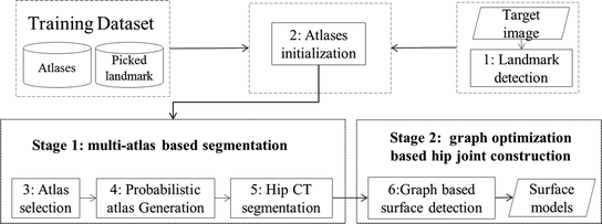
Fig. 2

The flowchart of our proposed segmentation method

2 Multi-atlas Based Hip CT Segmentation

2.1 Landmark Detection Based Atlas Initialization and Selection

In landmark detection step, totally 100 anatomical landmark positions are defined, in which 50 for pelvic model and 25 for each proximal femoral model. We apply landmark detector training and landmark prediction separately for each landmark position. For details, we refer to [19].

In atlas initialization step, using the detected N _lanatomical landmarks, paired-point scaled rigid registrations are performed to align all the N atlases to the target image space. Here, following the Algorithm 1 and 2 we speed up the scaled rigid registrations by aligning all the atlases and the target image to the same reference image, which is randomly selected as one of the training images. Since all the atlases have already been aligned to the reference image prior to the segmentation phase (Algorithm 1), we only need to transform target image to the reference space (Algorithm 2). Based on the scaled rigid registration results, we select N _satlases with the least paired-point registration errors for the given target image. The selected N _satlases are then registered to the target image using a discrete optimization based non-rigid registration [20].

2.2 Atlas-Based Segmentation

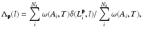
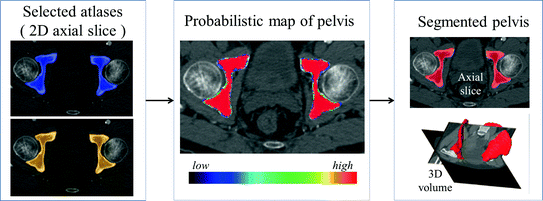
In this step, we first use the selected N _satlases after registration to generate probabilistic atlas (PA) both for background and hip joint structures (Fig. 3). We then formulate the multi-atlas based segmentation problem as a Maximum A Posteriori (MAP) estimation which can be efficiently solved using a graph cut based optimization method [21]. Using the known label of the selected atlases, PA of the target image ${\fancyscript{T}}$ is computed as:

${\Lambda_{\bf{p}}}(l) = \sum\limits_i^{N_s} \omega ({A_i}, {\fancyscript{T}})\delta (L_i^{\bf{p}},l)/\sum\limits_i^{N_s} \omega ({A_i}, {\fancyscript{T}}),$

(1)

where

$\delta (l,l^{\prime}) = \left\{ {\begin{array}{*{20}l} 1 \hfill & {{\kern 1pt} \text{if}\,l = l^{\prime}} \hfill \\ 0 \hfill & {{\kern 1pt} \text{otherwise}.} \hfill \\ \end{array} } \right.$

(2)

Fig. 3

Example of generating PA for segmentation. Left After non-rigidly registered two selected atlases to the target space. Middle Generated PA. Right Segmented pelvis

Here, i indicates the selected atlases, p denotes the voxel in the CT image, l represents the label of organ regions, $L_{i}^{{\mathbf{p}}}$ is the label of the voxel p in the atlas A _iand $\Lambda _{{\mathbf{p}}} (l)$ is probability that voxel p labeling as l. $\omega ({A_i},{\fancyscript{T}})$ is the weight of atlas A _iwhich is evaluated by the similarity between atlases and the target image. We use the normalized cross correlation (NCC) as the similarity between atlases and the target image. The probability $\Lambda_{{\mathbf{p}}} (l)$ is calculated for every voxels in the target image for background (where l = 0), pelvis (where l = 1), left femur (where l = 2), and right femur (where l = 3), respectively. For the given target image, a voxel-wise MAP estimation is defined as

$L_{{\mathbf{p}}} = { \arg }\mathop { \hbox{max} }\limits_{l} P(l|I_{{\mathbf{p}}} )$

(3)

where L _pis the given label of the voxel p, I _pis the intensity of p, l is the label of each region, and $P(l|I_{{\mathbf{p}}} )$ is the posterior probability. The MAP estimation aims to find a label l which can maximize the posterior probability. In other words, for a voxel p which has intensity I _p, if the label l of any region can maximize the posterior probability, the voxel will be assigned a label of l. The posterior probability is computed according the Bayes theory as 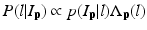$P(l|I_{{\mathbf{p}}} ) \propto p(I_{{\mathbf{p}}} |l)\Lambda_{{\mathbf{p}}} (l)$ , where $\Lambda _{{\mathbf{p}}} (l)$ is the PA describing the prior probability and $p(I_{{\mathbf{p}}} |l)$ is the conditional probability that is computed as we did in [22]. The MAP estimation is then solved with the graph cut method [21]. Giving the cost function of

$E(C) = \sum\limits_{{\mathbf{p}} \in {\fancyscript{T}}} {{D_{\mathbf{p}}}} ({C_{\mathbf{p}}}) + \lambda \sum\limits_{{\mathbf{p}},{\mathbf{q}} \in {N_{\mathbf{p}}}} {{V_{{\mathbf{p, q}}}}} ({C_{\mathbf{p}}},{C_{\mathbf{q}}})$

(4)

where C is the unseen labelling of target image; p and q the voxels in the target image; and N _pthe set of neighbors of voxel p. The date term of D _p(C _p) is defined based on the estimated posterior probability of $P(l|I_{{\mathbf{p}}} )$ . The relationships between a voxel and its neighborhoods are represented by the smoothness term $V_{{({\mathbf{p}},{\mathbf{q}})}} (C_{{\mathbf{p}}} ,C_{{\mathbf{q}}} )$ . Factor λ balances the influence of the two terms. The data term is defined as

$D_{{\mathbf{p}}} (C_{{\mathbf{p}}} ) = - \gamma {\ln\Lambda }_{{\mathbf{p}}} (l) - (1 - \gamma )\text{ln}p(I_{{\mathbf{p}}} |l)$

(5)

which measures the disagreement between a prior probabilistic (PA in our case) and the observed data (conditional probability) with a factor γ. The smoothness term is defined as

$V_{{{\mathbf{p}},{\mathbf{q}}}} (C_{{\mathbf{p}}} ,C_{{\mathbf{q}}} ) = \left\{ {\begin{array}{*{20}l} 0 \quad\hfill & {{\text{if}}\;C_{{\mathbf{p}}} = C_{{\mathbf{q}}} } \hfill \\ {\frac{1}{{(1 + |I_{{\mathbf{p}}} - I_{{\mathbf{q}}} |dist({\mathbf{p}},{\mathbf{q}}))}}},\quad \hfill & {{\text{otherwise}} .{\kern 1pt} } \hfill \\ \end{array} } \right.$

(6)

where dist(p, q) the Euclidean distance between two voxels. From these equations, we can find that V _(p,q)(C _p,C _q) becomes large when the distance between p and q is smaller and closer. Hence, two neighborhoods with the large cutting cost is large and they are not separated.

3 Graph Optimization Based Hip Joint Construction

3.1 Problem Formulation

After the multi-atlas segmentation of the hip joint region, we need to refine the segmented region and recover the hip joint structure by separating the surfaces of the acetabulum and the femoral head. In the CT image space, both the acetabulum and the femoral head are ball-like structures and their surfaces can be approximately represented as half-spherically shaped models. To separate these two surfaces, directly applying graph optimization-based surface detection in the CT image space as described in [13] would be an option. However, construction of a graph in the original CT image is not straightforward and requires finding correspondences between two adjacent surfaces obtained from a rough segmentation stage as done in [13], which is challenging.

In our method, instead of performing surface detection in the original CT image space, we first define a hip joint area in the extracted surface models of both the pelvis and the proximal femurs, and then unfold this area using a spherical coordinate transform as shown in Fig. 4. Since the spherical coordinate transform converts a half-spherically shaped surface to a planar surface, the surfaces of the acetabulum and the femoral head can therefore be unfolded to two terrain-like surfaces with a gap (joint space) between them as shown in Fig. 4. We reach this goal with following steps:

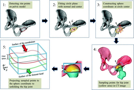
Fig. 4

A schumatic illustration of defining and unfolding a hip joint. Please see text in Sect. 3.1 for a detailed explanation

Detecting rim points of the acetabulum from segmented surface model of the pelvis using the method that we developed before [23] (Fig. 4: 1).

Fitting a circle to the detected rim points, determining radius R _cand center of the circle, as well as normal (towards acetabulum) to the plane where the fitted circle is located (Fig. 4: 2).

Constructing a spherical coordinate system as shown in Fig. 4: 3, taking the center of the fitted circle as the origin, the normal to the fitted circle as the fixed zenith direction, and one randomly selected direction on the plane where the fitted circle is located as the reference direction on that plane. Now, the position of a point in this coordinate system is specified by three numbers: the radial distance R of that point from the origin, its polar angle Θ measured from the zenith direction and the azimuth angle Φ measured from the reference direction on the plane where the fitted circle is located.

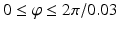
Sampling points in the spherical coordinate system from the hip joint area (see Fig. 4: 4) using a radial resolution of 0.25 mm and angular resolutions of 0.03 radians (for both polar and azimuth angles). Furthermore, we require the sampled points satisfying following conditions:

$\left\{ {\begin{array}{*{20}l} {R_{c} + 20 \le r \le R_{c} /2} \\ {0 \le \theta \le \pi /2} \\ {0 \le \varphi \le 2\pi } \\ \end{array} } \right.$

(7)

Getting corresponding intensity values of the sampled points from the CT image, which finally forms an image volume $I(\theta ,\varphi ,r)$ (Fig. 4: 5), where $0 \le r \le (20 + \frac{{R_{c} }}{2})/0.25$ , $0 \le \theta \le \pi /0.06$ , $0 \le \varphi \le 2\pi /0.03$ . The dimension of r depends on the radius of the fitted circle while the dimensions of θ and φ are fixed. To easy the description later, here we define the dimension of r as D _r.

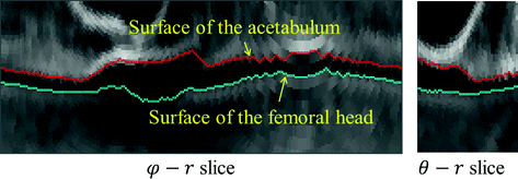
Figure 5 shows an example of generated volume $I(\theta ,\varphi ,r)$ of a hip joint. With such an unfolded volume, graph construction and optimal multiple-surface detection will be straightforward when the graph optimization-based multiple-surface detection strategy as introduced in the [12, 13] is used.

Fig. 5

An example of unfolded volume $I(\theta ,\varphi ,r)$ of a hip joint, visualized in 2D slices. Left A 2-D φ-r slice. Right A 2-D θ-r slice. In both slices, the green line indicates the surface of the femoral head and the red line indicates the surface of the acetabulum. The gap between these two surface corresponds to the joint space of the hip (Color figure online)

3.2 Graph Construction for Multi-surface Detection

For the generated volume $I(\theta ,\varphi ,r)$ as shown in Fig. 5, we assume that r is implicitly represented by a pair of ( $\theta ,\varphi$ ), e.g. $r = f(\theta ,\varphi )$ . For a fixed ( $\theta ,\varphi$ ) pair, the voxel subset $\{ I(\theta ,\varphi ,r)|0 \le r < R\}$ forms a column along the $$r$$

-axis and is defined as Col(p). Each column has a set of neighbors and in this paper 4-neighbor system is adopted. The problem is now to find k coupled surfaces such that each surface intersects each column exactly at one voxel. In our case, we expect to detect two adjacent surfaces of a hip joint, i.e., the surface of the acetabulum S _aand the surface of the femoral head S _f. To accurately detect these two surfaces using graph optimization-based approach, following geometric constraints need to be considered:

For each individual surface, the shape changes of this surface on two neighboring columns Col(p) and Col(q) are constrained by smoothness conditions. Specifically, if Col(p) and Col(q) are neighbored columns along the $\theta$ -axis, for each surface S (either S _aor S _f), the shape change should satisfy the constraint of $|S(p) - S(q)| = |r_{p} - r_{q} | \le\Delta _{\theta }$ , where $r_{p} = p(\theta_{1} ,\varphi )$ and $r_{q} = q(\theta_{2} ,\varphi )$ are coordinate values of surface S (either S _aor S _f) intersecting columns Col(p) and Col(q), respectively. The same constraint should also be applied along the $\varphi$ -axis with a smoothness parameter $\Delta _{\varphi }$ .