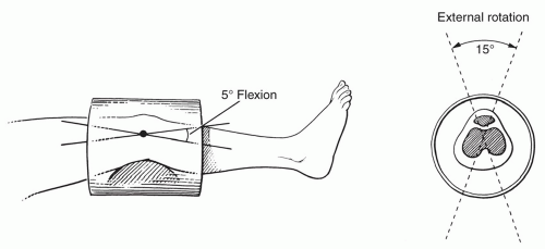
 Figure 7.1 Knee positioned in a volume coil. The knee is flexed 5° to 10° and can be externally rotated 15°. |
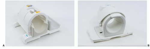 Figure 7.2 Volume knee coils (A and B). (Courtesy of Siemens Medical Systems, Erlangen, Germany.) |
disadvantage of requiring longer acquisition times, and the long TE T2-weighted images are technically demanding in terms of imager performance.
Table 7.1 MR Screening Examination of the Knee at 1.5 T | ||||||||||||||||||||||||||||||||||||||||||||||||||||||||||||||||||||||||||||||||||||||||||||||||||||||||||||
|---|---|---|---|---|---|---|---|---|---|---|---|---|---|---|---|---|---|---|---|---|---|---|---|---|---|---|---|---|---|---|---|---|---|---|---|---|---|---|---|---|---|---|---|---|---|---|---|---|---|---|---|---|---|---|---|---|---|---|---|---|---|---|---|---|---|---|---|---|---|---|---|---|---|---|---|---|---|---|---|---|---|---|---|---|---|---|---|---|---|---|---|---|---|---|---|---|---|---|---|---|---|---|---|---|---|---|---|---|
| ||||||||||||||||||||||||||||||||||||||||||||||||||||||||||||||||||||||||||||||||||||||||||||||||||||||||||||
special capabilities for depicting chondral and osteochondral lesions as shown in these images, but these have not been fully explored as yet.
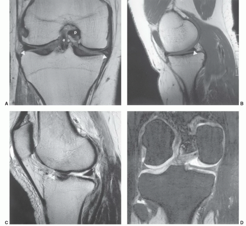 Figure 7.3 A: Coronal SE 450/15 image of the knee demonstrates normal signal intensity in the marrow. The menisci are low signal intensity and the articular cartilage is intermediate signal intensity. The cruciate ligaments (a, anterior; p, posterior) are seen in the intercondylar notch. The collateral ligaments (arrowheads) are also low signal intensity. B: Sagittal proton density (2,300/26) image of the posterior medial knee demonstrates the posterior horn of the medial meniscus with intrasubstance increased signal intensity (arrowhead), but not communication with the articular surface. C: Sagittal fast spin-echo T2-weighted sequence (3,300/80) image of the knee demonstrates abnormal signal and truncation of the anterior horn and body of the lateral meniscus (arrowhead). D: Coronal dual-echo steady-state image (three-dimensional, 23.87/6.73) demonstrates normal meniscal signal intensity and excellent cartilage detail. |
for isotropic resolution in three-dimensional imaging. This is imposed by the short repetition time that must be used.
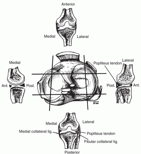 Figure 7.4 Axial anatomy of the knee and selected coronal and sagittal sections. |
60% to 80% water. Collagen makes up 50% of the weight of cartilage and proteoglycans contribute 30% to 35%.52,66
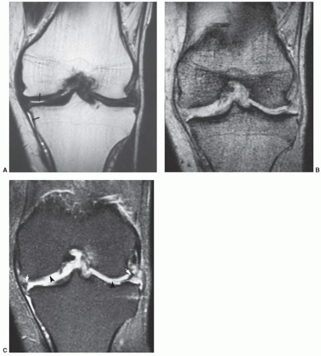 Figure 7.5 Coronal images of the knee with the same plane of section in a patient with meniscal tears and articular cartilage loss. A: Fast spin-echo (4,000/108) is similar in appearance to a T1-weighted spin-echo sequence (marrow and fat have high signal intensity) except for high signal intensity of joint fluid and vessels (arrows). Other intra-articular structures are not clearly defined. Gradient echo (700/31, flip angle 25°) (B) and fat-suppressed spin-echo (SE 2,000/80) (C) images demonstrate the meniscal tears (arrows) and loss of articular cartilage (arrowheads) more clearly. |
and tibial condyles (Fig. 7.20). The patella is divided into several Wiberg types. The medial and lateral facets are of equal size in type I. Type II, the most common configuration, has a smaller medial than lateral facet (Fig. 7.10). Type III has a very small medial facet that is convex and a large, concave lateral facet. Both facets are covered with hyaline cartilage and most easily seen on axial MR images (Fig. 7.10).64,70,71
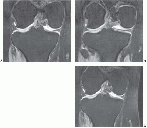 Figure 7.6 Three-dimensional gradient-echo images (A-C) of the knee from posterior to anterior demonstrating superior cartilage detail. |
Along the medial, lateral, and posterior aspects of the capsule, the synovial membrane attaches to the femur at the edges of the articular surfaces posteriorly. Medially and laterally, it passes from the articular margins inferiorly to attach to the articular margins of the tibial condyles (Fig. 7.14D). The intrasynovial space that extends from the intracondylar fossa superiorly to the intracondylar area of the tibia inferiorly houses the cruciate ligaments. The cruciate ligaments are, therefore, covered superiorly, medially, laterally, and anteriorly by synovial membrane but not posteriorly (Fig. 7.14A, B, and E). Posterolaterally, the synovial membrane is separated from the fibrous capsule by the popliteus tendon. It is not unusual to identify a bursa along the popliteus tendon that communicates with the joint space posterolaterally. The other common bursae about the knee are listed in Table 7.2 (Fig. 7.15).19,65 There is also a lateral synovial extension that may be implicated in iliotibial band syndrome.73
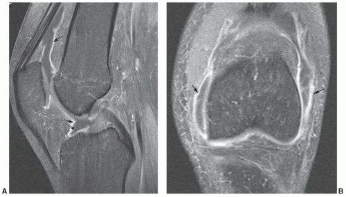 Figure 7.7 Sagittal (A) and anterior coronal (B) intravenous post-contrast fat-suppressed T1-weighted images demonstrating synovial enhancement (arrows). Due to the early imaging the synovial fluid has not enhanced on the sagittal image (A). There is early enhancement of synovial fluid on the coronal image performed two sequences later in the examination. |
Table 7.2 Bursae About the Knee | ||||||||||||||||||||||||||||||||||||||||||||||||
|---|---|---|---|---|---|---|---|---|---|---|---|---|---|---|---|---|---|---|---|---|---|---|---|---|---|---|---|---|---|---|---|---|---|---|---|---|---|---|---|---|---|---|---|---|---|---|---|---|
| ||||||||||||||||||||||||||||||||||||||||||||||||
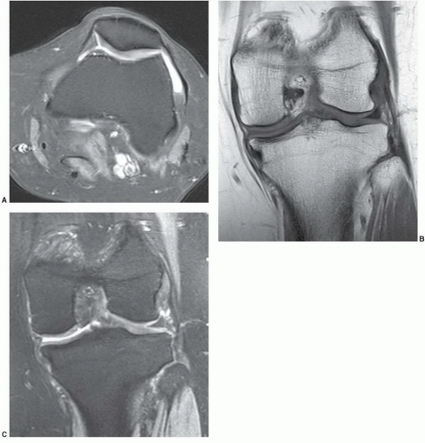 Figure 7.8 Screening examination of the knee performed at 1.5 T. A: Axial images are obtained using a turbo spin-echo proton density fat-suppressed sequence (2,480/28, ET 3). Coronal images are obtained using turbo spin-echo T1-weighted (800/11, ET 3) (B) and the second coronal sequence using DESS (19.6/5.47, ET 1) (C). Sagittal sequences include turbo spin-echo proton density (BLADE, 2,850/42, ET 9) with fat saturation (D) and the same sequence without fat saturation (E). |
the popliteal muscle and tendon.84 The coronary ligament, ligament of Winslow, and lateral collateral ligament are secondary restraints.65
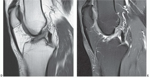 Figure 7.8 (continued) |
suggested that the orientation of the layers explains the origin of most meniscal tears as they appear to align with the axis of the collagen fibers.89 The fibrocartilaginous menisci have a differing shape, with the medial meniscus being larger and thicker in transverse diameter posteriorly than anteriorly (Figs. 7.11, 7.13, and 7.15A). The lateral meniscus is more C-shaped and uniform in width (Fig. 7.15A). Despite the difference in shape, the medial meniscus covers less articular surface (50%) compared with 70% coverage by the lateral meniscus.89 There are several ligamentous attachments that may cause confusion on MR images. For example, the posterior horn of the lateral meniscus is closely applied to the PCL and may give off a band of fibers, termed the meniscofemoral ligament, that follows the PCL to its attachment on the femur. Between the anterior horns of the medial and lateral meniscus there is a transverse band of fibers termed the transverse ligament of the knee. This can easily be confused with an anterior meniscal tear, especially on the medial side (Fig. 7.16).64,65 Another variant, the meniscomeniscal ligament, may also be confused with meniscal pathology. The medial meniscomeniscal ligament extends from the anterior horn of the medial meniscus to the posterior horn of the lateral meniscus. The lateral meniscomeniscal ligament extends from the anterolateral to posteromedial meniscus.90 The central attachments of both menisci are defined as the anterior and posterior root ligaments.89
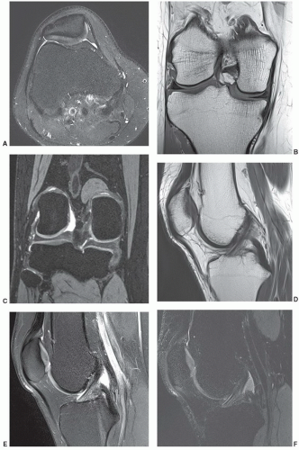 Figure 7.9 Screening examination of the knee performed at 3.0 T (A). Axial images are obtained using a turbo spin-echo proton density sequence (4,614/61, ET 7). Coronal images are obtained using a turbo spin-echo T1-weighted (800/11, ET 2) (B) and DESS sequence (14.59/5.03, ET 2) (C). The first saggital sequence is a turbo spin-echo proton density sequence (3,370/40, ET 7) (D), followed by a similar sequence with fat suppression (E) sagittal STIR (F). |
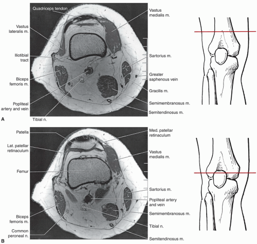 Figure 7.10 Axial SE 500/15 MR images through the knee with level of section demonstrated. A: Axial image through the distal femoral shaft above the patella. B: Axial image through the upper patella. C: Axial image through the upper femoral condyles and patella. D: Axial image through the femoral condyles and lower patella. E: Axial image through the lower femoral condyles below the patella. F: Axial image and illustration through the upper tibia. G: Axial image and illustration through the tibia and fibular head. H: Axial image through the upper tibia and fibula. |
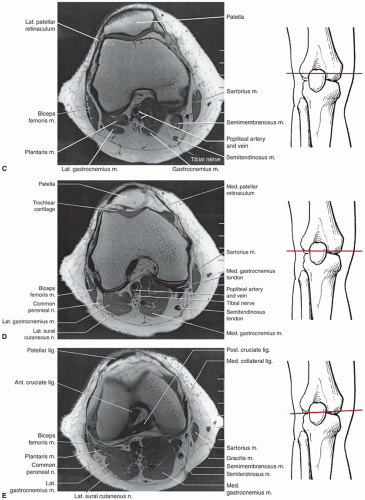 Figure 7.10 (continued) |
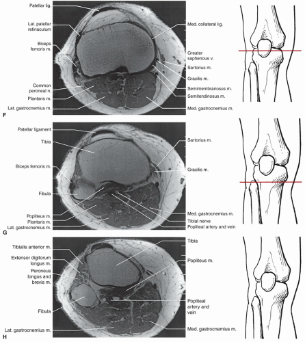 Figure 7.10 (continued) |
posterior suprapatellar fat pad anterior to the femur (Fig. 7.16).91,92 Hoffa fat pad is bordered by the inferior pole of the patella superiorly, the patellar tendon anteriorly, the joint capsule posteriorly, and the deep infrapatellar bursa inferiorly.91 The transverse ligament can be seen in the posterior aspect of Hoffa fat pad (Fig. 7.17).91,92
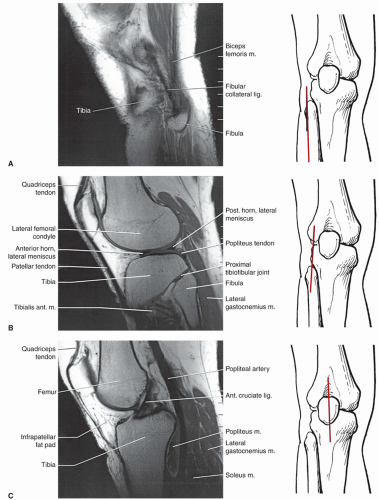 Figure 7.11 Sagittal SE 500/15 images of the knee from lateral to medial with plane of section demonstrated. A: Sagittal image through the lateral margin of the fibular head. B: Sagittal image through the fibular head. C: Sagittal image through the anterior cruciate ligament. D: Sagittal image through the posterior cruciate ligament. E: Sagittal image through the medial compartment. F: Sagittal image through the medial soft tissues and margin of the femoral condyle. |
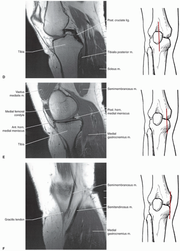 Figure 7.11 (continued) |
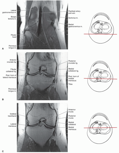 Figure 7.12 Coronal SE 500/15 images of the knee from posterior to anterior with level of section demonstrated. A: Coronal image through the soft tissues and fibular head. B: Coronal image through the posterior tibia and femoral condyles. C: Coronal image through the mid-joint. D: Coronal image through the anterior joint. |
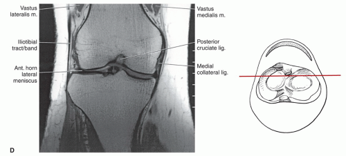 Figure 7.12 (continued) |
does not create as much motion artifact as when the patient is supine.2
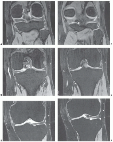 Figure 7.13 Coronal DESS three-dimensional (23.87/6.73, field of view 14 cm, matrix 256 × 192, two acquisitions) images (A-F) of the knee demonstrating both medial and lateral menisci and superior cartilage detail. |
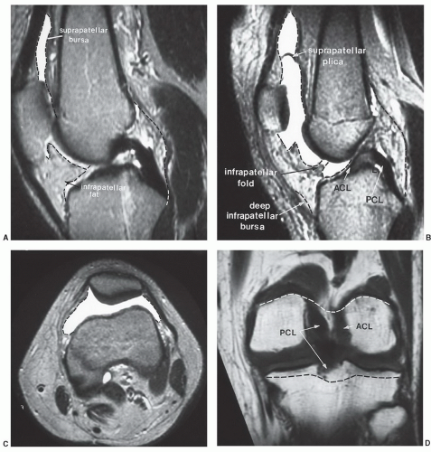 Figure 7.14 MR images of the knee demonstrating the synovial and capsular attachments (broken lines) of the knee. A: Sagittal image in the plane of the posterior cruciate ligament. B: Sagittal image in the plane of the anterior cruciate ligament. C: Axial image at the patellar level demonstrating the synovial reflection (broken lines). D: Posterior coronal image demonstrating the posterior synovial and capsular margins (broken lines). E: Axial image of the tibial articular surface demonstrating meniscal and cruciate attachments and synovial reflections. ACL, anterior cruciate ligament; PCL, posterior cruciate ligament. |
Shellock et al.100 reported an increase in hematopoietic marrow in 43% of marathon runners, compared with only 15% of patients with knee disorders and 3% of normal healthy patients. This marrow conversion pattern may be due to “sports anemia,” which has been attributed to numerous problems such as hemolysis, hematuria, increased plasma volume, and gastrointestinal blood loss.100
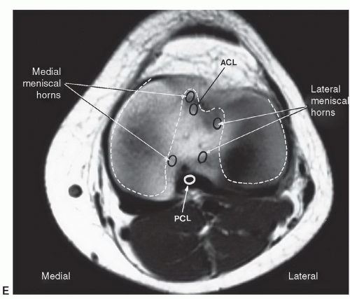 Figure 7.14 (continued) |
Table 7.3 Knee Flexors and Extensors | |||||||||||||||||||||||||||||||||||||||||||||||||||||||||||||||||
|---|---|---|---|---|---|---|---|---|---|---|---|---|---|---|---|---|---|---|---|---|---|---|---|---|---|---|---|---|---|---|---|---|---|---|---|---|---|---|---|---|---|---|---|---|---|---|---|---|---|---|---|---|---|---|---|---|---|---|---|---|---|---|---|---|---|
| |||||||||||||||||||||||||||||||||||||||||||||||||||||||||||||||||
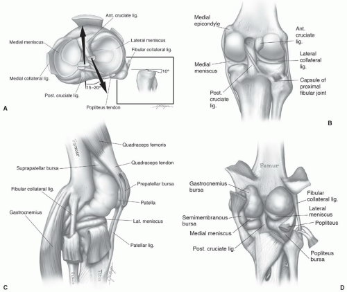 Figure 7.15 Axial (A), coronal (B), sagittal (C), and posterior (D) illustrations of the ligaments, menisci, and bursae of the knee. |
Table 7.4 Common Variants and Artifacts in MR Imaging of the Knee | ||||||||||||||||||
|---|---|---|---|---|---|---|---|---|---|---|---|---|---|---|---|---|---|---|
| ||||||||||||||||||
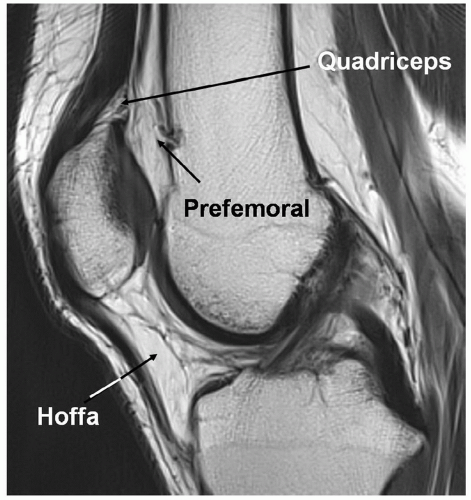 Figure 7.16 Fat pads of the anterior knee. Saggital T1-weighted 3.0-T MR image demonstrating the three anterior fat pads of the knee. |
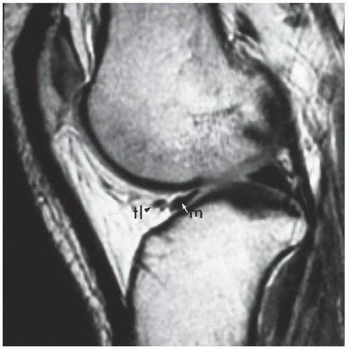 Figure 7.17 Sagittal T1-weighted image of the knee demonstrating a normal anterior horn of the medial meniscus (m, arrow) and the transverse ligament (tl, arrowhead). This should not be confused with a meniscal tear. |
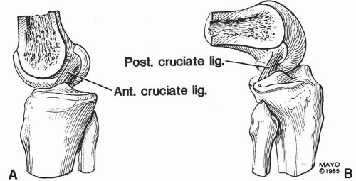 Figure 7.18 Sagittal illustrations of the knee and cruciate ligaments in the extended (A) and flexed (B) positions. |
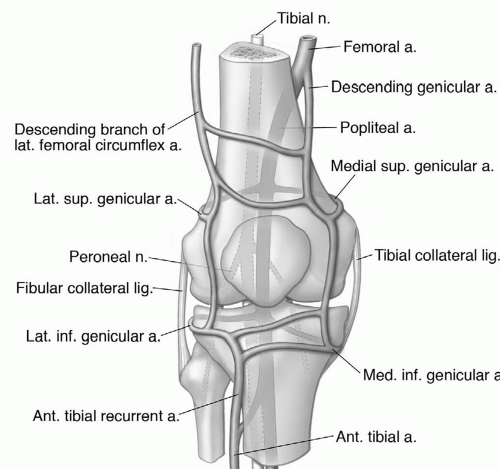 Figure 7.19 Neurovascular anatomy of the knee. |
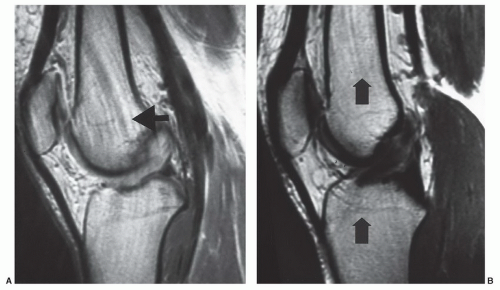 Figure 7.20 A: Sagittal proton density image of the knee demonstrating pulsatile motion artifact from the popliteal artery. The phase encoding is in the anteroposterior direction (arrow). Artifact is decreased (B) by switching the phase encoding to the superior-inferior (arrows) direction. |
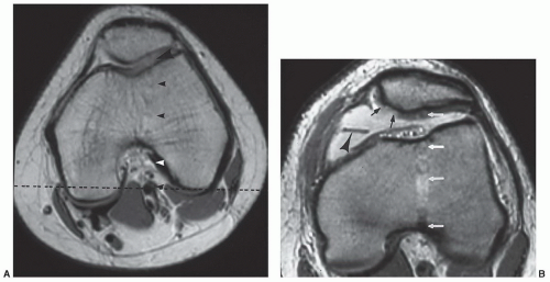 Figure 7.21 A: Axial proton density image in a patient referred for patellofemoral pain. The focal defect in the lateral femoral condyle (large arrowhead) is due to flow artifact (small arrowheads). This should not be confused with an articular defect. This problem can be avoided by swapping phase direction to the transverse (dotted line) plane. B: Axial T2-weighted image through the patellofemoral compartment. There is an effusion, a medial plica (arrowhead), and grade IV chondromalacia on the medial patellar facet (small arrows). Flow artifact (white arrows) with phase encoding in the anteroposterior direction creates a false lesion (increased signal) in the lateral facet. |
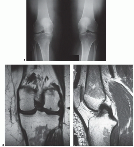 Figure 7.22 Normal male athlete. A: Anteroposterior radiographs of the knees demonstrate normal marrow and medial compartment narrowing. T1-weighted coronal (B) and sagittal (C) images show decreased signal intensity in the femoral metaphysis and diaphysis and upper tibia due to red marrow reconversion. |
completely identified. Normal variations in the posterior ligaments can be confused with partial tears in the PCL, a meniscal tear, or osteochondral fragment.110,111,112 Themeniscal femoral ligament extends from near the posterior capsular attachment of the lateral meniscus to the medial femoral condyle and may have two branches. The most common segment is the ligament of Wrisberg that is seen just posterior to the PCL (Fig. 7.28). This is evident in 23% to 32.5% of sagittal MR images and should not be confused with a partial tear.93,96,103,104,112 The anterior bundle of this ligament or the ligament of Humphrey is seen in 34% of patients (Fig. 7.29).96,103 This lies just anterior to the PCL.
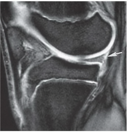 Figure 7.23 Sagittal gradient-echo image of the posterior medial meniscus demonstrating increased signal intensity at the meniscosynovial junction (arrow), which can be confused with a tear. |
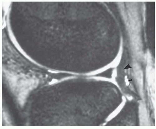 Figure 7.24 Sagittal gradient-echo image of the knee. The popliteus tendon (large arrowhead) and tendon sheath pass between the lateral meniscus and capsule. This should not be mistaken for a meniscal tear. The small areas of high signal intensity (small arrowhead) are due to the inferior genicular vessels. |
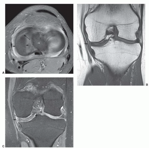 Figure 7.25 Discoid medial meniscus. A: Axial fat-suppressed proton density image demonstrating the size of the discoid meniscus (short arrows) with a tear (long arrow) anteriorly. Coronal T1-weighted (B) and DESS (C) images demonstrating the extension of the meniscus into the joint (short arrows). |
patients with trauma or suspected internal derangement of the knee.3,21,81,89,114,115,116,117,118
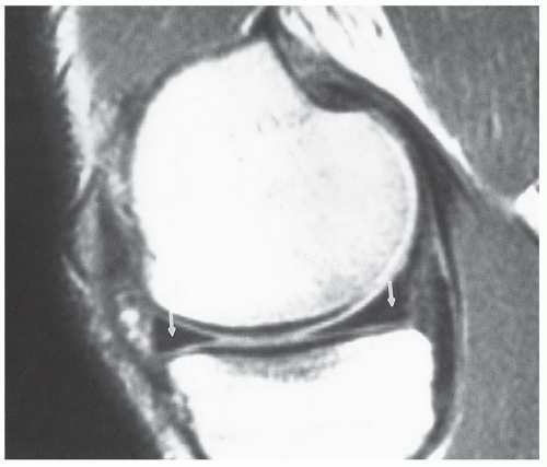 Figure 7.26 Sagittal proton density image of the knee using a 128 × 256 matrix and 16-cm field of view. The phase encoding is in the superior-inferior direction. The truncation artifact creates a faint linear area of increased signal intensity approximately 2 pixels from the meniscal margin (arrows). |
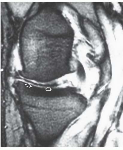 Figure 7.27 Oblique radial gradient-echo image showing an irregular low-intensity structure (open arrows) extending into the joint from the meniscal margin due to vacuum phenomenon. |
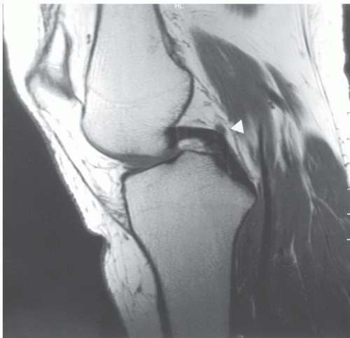 Figure 7.28 Sagittal proton density-weighted image demonstrating a normal posterior cruciate ligament. The ligament of Wrisberg (arrowhead) should not be confused with a posterior cruciate defect. |
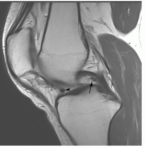 Figure 7.29 Sagittal T1-weighted image of the posterior cruciate ligament. Note the ligament of Humphrey (arrow) anteriorly that should not be confused with a posterior cruciate abnormality. There is also a prominent transverse ligament (arrowhead) anteriorly at the posterior margin of Hoffa fat pad. |
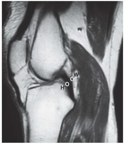 Figure 7.30 Sagittal proton density-weighted MR image demonstrating the usual locations of the meniscofemoral ligaments of Humphrey (H) and Wrisberg (W). |
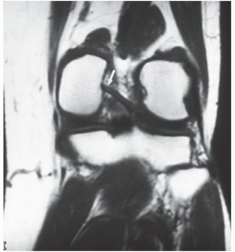 Figure 7.31 Coronal T1-weighted image demonstrating a type I meniscofemoral ligament inserting on the medial femoral condyle (arrow). |
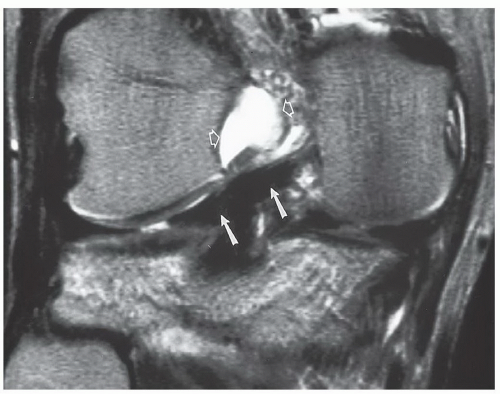 Figure 7.32 Coronal T2-weighted image demonstrating a type II meniscofemoral ligament (arrows) that is less vertically oriented than the type I in Fig. 7.31. There is high signal intensity in the notch (open arrows) due to an ACL tear. |
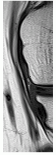 Figure 7.33 Focused coronal T1-weighted image of the medial collateral ligament demonstrating a linear fat plane (arrow) between the deep and superficial segments. |
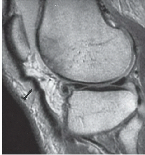 Figure 7.34 Sagittal proton density-weighted image demonstrating buckling of the patellar tendon (arrow) due to the extended position of the knee. |
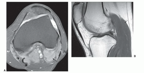 Figure 7.35 Accessory gastrocnemius. Axial fat-suppressed proton density (A) and sagittal T1-weighted (B) images demonstrating an accessory lateral head of the gastrocnemius (arrow). |
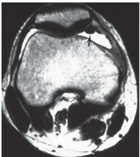 Figure 7.36 Axial T2-weighted image of the knee in a patient with knee pain. There is an effusion with a low-signal-intensity structure (arrow) medially. This could be mistaken for a loose body, medial patellar fragment, or thickened soft tissue structure. The signal abnormality was created by an air collection from arthroscopy 2 days earlier. |
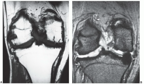 Figure 7.37 Patient with advanced osteoarthritis and a low-signal-intensity defect medially (arrows). The artifact is subtle on the coronal T1-weighted image (A) and more obvious on the gradient-echo image (B). This artifact was created by a small metal remnant from previous arthroscopy. |
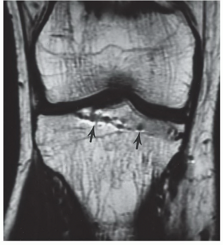 Figure 7.38 Coronal T1-weighted image, demonstrating artifacts from a previous screw tract (arrows) created by residual microscopic metal fragments. |
posterior to the anterior.61 Chronic repetitive trauma is common both in athletes and nonathletes with aging.75,125 Chrondrocyte necrosis and increase in mucoid ground substance can lead to meniscal tears.126
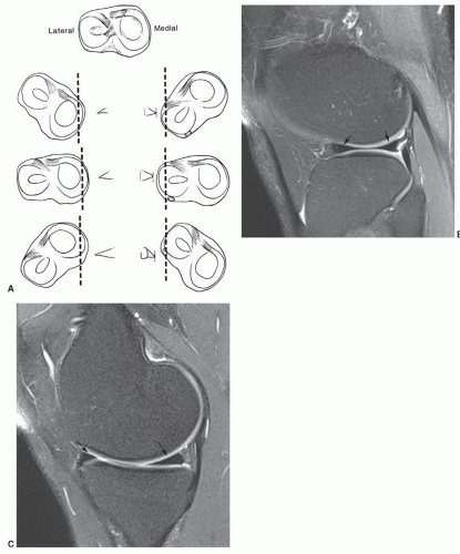 Figure 7.39 A: Tangential sections of the medial and lateral meniscus. (From Rand JA, Berquist TH. The knee. In: Berquist TH, ed. Imaging of Orthopedic Trauma. 2nd ed. New York, NY: Raven Press; 1992:333-432.) B: Sagittal turbo spin-echo fat-suppressed proton density-weighted image of the knee through the lateral meniscus demonstrating the similar size of the anterior and posterior horns (arrows). C: Sagittal turbo spin-echo fat-suppressed proton density-weighted image through the medial meniscus demonstrating the posterior horn is significantly larger than the anterior horn (arrows). |
on the second echo of spin-echo sequences. Today, turbo or FSE proton density sequences are commonly used with or without fat suppression.89,129,130 The increased signal intensity seen on proton density MR images is felt to be related to hydrogen protons attached to macromolecules in the region of the tear.89 There is still some controversy regarding the accuracy of conventional spin-echo and FSE proton density sequences. Rubin et al.41 found similar sensitivities and specificities with both conventional and FSE techniques. If using FSE techniques, Rosas and De Smet89 recommend lower echo train lengths (<4) and larger bandwidths (>30 mHz) to reduce blurring. We currently obtain FSE proton density sagittal images with and without fat suppression. False negatives can be reduced using fat-suppression techniques (Fig. 7.42).129,130 Statistics for fat-suppressed proton density FSE sequences result in 92% to 95% sensitivity, 92% to 93% specificity, and 92% to 93% accuracy.130
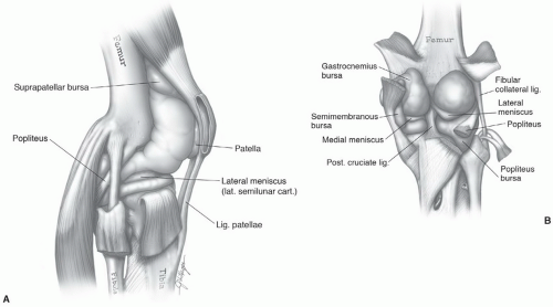 Figure 7.40 Lateral (A) and posterior (B) illustrations of the knee demonstrating the joint space and associated ligament and meniscal anatomy. |
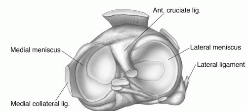 Figure 7.41 Menisci and their attachments and associated ligament and tendon anatomy. |
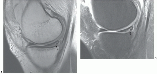 Figure 7.42 Sagittal proton density fast spin-echo without (2,000/25, ET 5, 4-mm thick sections) (A) and with fat suppression (3,000/37, ET 5, 4-mm thick sections) (B) demonstrating the increased conspicuity of the peripheral medial meniscal tear communicating with the inferior articular surface (arrow) on the fat-suppressed image (B). |
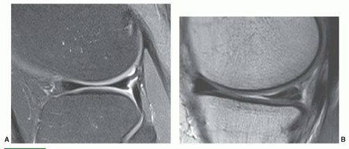 Figure 7.43 Normal and abnormal menisci. A: Normal 3.0-T sagittal turbo spin-echo fat-suppressed proton density-weighted image of the lateral meniscus. There is no signal in the meniscus. Note the popliteus tendon and sheath posteriorly. B: Grade 2 globular increased signal intensity in the medial meniscus on a sagittal 3.0-T proton density-weighted image. C: Grade 3 increased signal intensity in the posterior horn of the medial meniscus communicating with the inferior articular surface on 1.5-T proton density image (small arrowhead). D: Sagittal 1.5-T gradient-echo image demonstrating a grade 3A tear (small arrowhead) with an associated meniscal cyst (large arrowhead). E: Sagittal 1.5-T gradient-echo image demonstrating a more complex linear tear in the posterior horn of the medial meniscus. F: Grade 3B meniscal tear with a broad area of articular involvement (arrowheads) on gradient-echo 1.5-T image. |
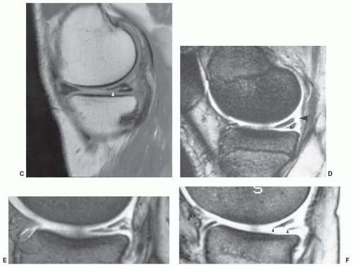 Figure 7.43 (continued) |
significant signal-intensity changes that communicate with the articular surface.
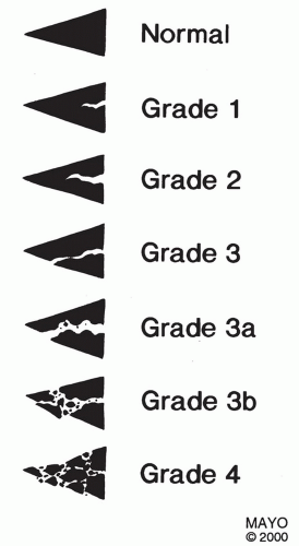 Figure 7.44 Meniscal tear grading system. |
 Figure 7.45 Sagittal 1.5-T proton density-weighted (A) and coronal three-dimensional DESS (B) images demonstrate complex degenerative tearing of the anterior horn and body of the lateral meniscus. Additionally, the coronal image B shows extrusion of the fragments (white arrowhead). |
flipped-fragment sign (Fig. 7.51) is seen with 44% of medial and 29% of lateral meniscal bucket-handle tears (Table 7.5).54 Another sign is a fragment in the intercondylar notch, which is not the same as the double-PCL sign.89 Defining a fragment in the notch may be difficult, especially when they are small and the configuration of the meniscus is not significantly truncated (Fig. 7.48; Table 7.5). Larger fragments are identified with 66% of medial and 43% of lateral meniscal tears.54 Detection may be improved by using coronal STIR images. Magee and Hinson48 reported detection of 93% of fragments using STIR sequences. Defining the fragments is important, as they need to be removed arthroscopically.48 The final sign is the absent “bow-tie sign,” which is seen as absence of the normal meniscal configuration on sagittal images through the meniscus (Fig. 7.52).89
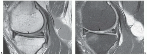 Figure 7.46 1.5-T proton density (A) and proton density with fat suppression (B) images of a complex medial meniscal tear with associated cartilage loss (arrow) and a large popliteal cyst. |
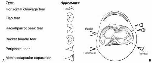 Figure 7.47 A: Types of meniscal tears. B: (1) Radial tear with cross-sectional appearance. (2) Horizontal tear that is only seen on tangential view. (3) Flap tear, oriented oblique to the long axis of the meniscus. Note the distance from the apex increases (a to b) as the tear extends into the meniscus. (4) Vertical tear. Meniscal tears seen tangentially. |
to find an associated meniscal cyst. The etiology of meniscal cysts is felt to be related to extension of joint fluid through the tear.89 Horizontal meniscal tears are more common in elderly patients with degenerative disease.89,147
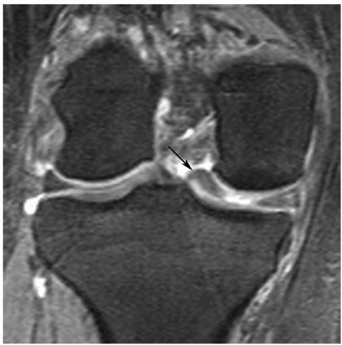 Figure 7.48 Bucket-handle tear with a displaced fragment in the intercondylar notch (arrow). |
Table 7.5 Bucket Handle Tears: MRI Features | ||||||||||||||||||
|---|---|---|---|---|---|---|---|---|---|---|---|---|---|---|---|---|---|---|
| ||||||||||||||||||
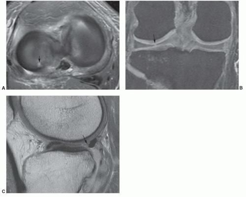 Figure 7.49 Radial tear in the posterior horn of the lateral meniscus. Axial fat-suppressed proton density 1.5 T (A), coronal DESS (B), and sagittal proton density-weighted (C) images demonstrate a focus of free edge increased signal intensity (arrows in A and B) and a truncated appearance at the level of the tear on the saggital image (arrow in C). |
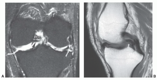 Figure 7.50 Coronal fat-suppressed T2-weighted image (A) demonstrating a medial tear (curved arrow) with a large displaced fragment (black arrow) that gives the appearance of two posterior cruciate ligaments (PCL). There is also a complex tear of the lateral meniscus (white arrow) and loss of articular cartilage. Sagittal proton density-weighted image (B) demonstrating a medial meniscal tear with a large displaced fragment (small arrow), resulting in a double-PCL sign. |
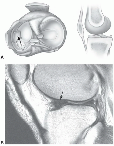 Figure 7.51 Flipped-fragment (large or double anterior horn) sign. A: Illustration of the flipped fragment sign seen in the axial and sagittal planes. B: Sagittal proton density-weighted MR image with a large anterior horn (arrow). A portion of the posterior horn is still evident. |
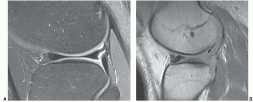 Figure 7.52 The absent bow-tie sign. A: Normal fat-suppressed turbo spin-echo proton density sagittal image demonstrating the normal bow-tie configuration of the meniscus. B: Sagittal proton density-weighted image demonstrating absence of the posterior portion of the bow tie (arrow). Note the double appearance of the anterior horn of the meniscus. |
chondrocyte nutrition. Stress to the articular cartilage is also reduced. The meniscus also restricts anterior displacement of the tibia on the femur, reducing stressonthe ACL.64,160,161
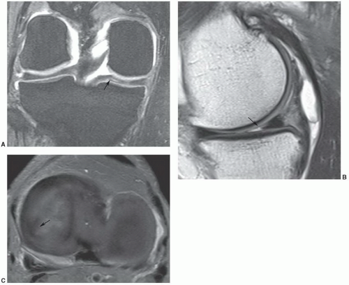 Figure 7.53 Parrot-beak tear. Coronal DESS (A), sagittal proton density (B), and axial fat-suppressed proton density (C) images demonstrate a radial tear extending peripherally (arrow). |
sequences are more useful in this setting as fluid signal intensity extending to the articular surface are more specific. Specificities have been reported as high as 90%.165 More recent studies suggest that the specificity ranges from 73% to 88% using the earlier criteria.89,162
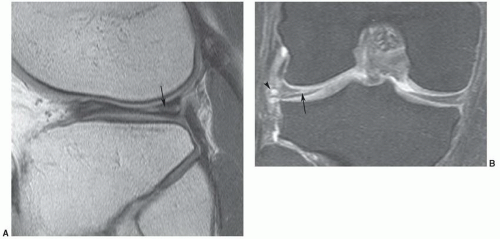 Figure 7.54 Horizontal tear of the lateral meniscus with an associated meniscal cyst. Sagittal proton density-weighted (A) and coronal DESS (B) images demonstrate a horizontal tear in the lateral meniscus (arrow) with an associated menical cyst (arrowhead). |
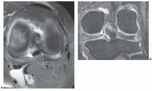 Figure 7.55 Meniscal root tear. Axial fat-suppressed proton density-weighted (A) and coronal DESS (B) images demonstrate a radial appearing posterior medial meniscal root tear (arrow). There is also a popliteal cyst with a loose body (arrowhead). |
arthrograms least accurate (58%) for evaluating menisci after surgical procedures.163 The use of arthrography remains somewhat controversial.89 In a recent study, De Smet et al.168 found that similar to the nonoperative knee, any signal intensity contacting the meniscal surface on two or more contiguous sections is most likely a new tear. This group reserves MR arthrography for patients with greater than 25% of the meniscus removed.168 We have not used MR arthrography except in selected cases or when specifically requested by the orthopedic surgeons. In our experience, MRI equivocal cases are most often reexamined arthroscopically.
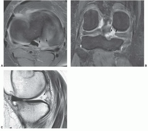 Figure 7.56 Medial meniscal root tear. Axial fat-suppressed proton density (A), coronal DESS (B), and sagittal proton density-weighted (C) images demonstrate a complete posterior medial mensical root tear (arrows). There is extrusion of the anterior meniscus (arrowhead in C). |
Table 7.6 MRI of Meniscal Tears | |||||||||||||||||||||||||||||||||||||||||||||||||||||||||||||||||||||||||||||
|---|---|---|---|---|---|---|---|---|---|---|---|---|---|---|---|---|---|---|---|---|---|---|---|---|---|---|---|---|---|---|---|---|---|---|---|---|---|---|---|---|---|---|---|---|---|---|---|---|---|---|---|---|---|---|---|---|---|---|---|---|---|---|---|---|---|---|---|---|---|---|---|---|---|---|---|---|---|
| |||||||||||||||||||||||||||||||||||||||||||||||||||||||||||||||||||||||||||||


