Interpretation of Magnetic Resonance Images

Mark S. Collins

Richard L. Ehman

Magnetic resonance imaging (MRI) is a powerful and versatile diagnostic tool utilized by radiologists and clinicians to provide definitive diagnoses for a wide range of musculoskeletal pathology. Compared to conventional radiographs, nuclear medicine studies, musculoskeletal computed tomography (CT), and ultrasound, MRI provides the best combined sensitivity and specificity for clinical differential diagnostic considerations, which include a broad spectrum of osseous, cartilage, and soft tissue pathology. The goals of the musculoskeletal imager include providing images that demonstrate excellent spatial resolution to evaluate complex soft tissue anatomy while still maintaining maximal signal-to-noise ratio. Most importantly, the ultimate goal is to demonstrate excellent conspicuity of pathology as compared to normal background structures to assist in making confident imaging diagnoses. This is accomplished by tailoring the imaging sequences to do the best evaluation of clinical diagnostic considerations and may include the use of intravenous or intra-articular gadolinium.

This chapter provides an overview of basic interpretation techniques that establish a confident imaging diagnosis. These techniques take into account inherent properties of normal and pathologic musculoskeletal tissues that are emphasized by MR tissue characterization. These physical properties may be accentuated by tailoring the MR examination to demonstrate the conspicuity of pathologic processes by applying the best combination of a multitude of available MR sequences. There are certainly many individual preferences utilized by experienced musculoskeletal imagers that may differ due to different magnet systems, coil design, and uniquely developed sequences appropriate for those systems. Regardless, the goal is the same: Obtaining the most accurate diagnosis possible, utilizing superior imaging techniques and thorough interpretation patterns.

BASIC IMAGE INTERPRETATION

Interpretation of MR images initially begins with differentiation of normal structures from pathologic processes. Pathologic processes of the musculoskeletal system are identified at MRI by abnormal morphology, abnormal signal characteristics, or the combination of both. An acute disruption of the anterior cruciate ligament of the knee is demonstrated by the presence of abnormal morphology (discontinuous or indistinct fibers, ligamentous laxity, and mass effect) and abnormal signal intensity (due to intra-substance hemorrhage or edema) (Fig. 2.1A). A chronic tear of a ligament may demonstrate abnormal morphology (ligament attenuation and laxity) with normal signal intensity (Fig. 2.1B). Figure 2.2 demonstrates a partial thickness intra-substance tear of the supraspinatus tendon, which has abnormal signal but grossly normal morphology.

Most non-lipomatous, solid, soft tissue masses have relatively nonspecific MR features that do not allow tissuespecific diagnoses. However, on occasion, careful evaluation of the morphology and internal signal characteristics of soft tissue masses can provide a definitive pre-biopsy histologic diagnosis. Figure 2.3 demonstrates two different cases of peripheral nerve sheath tumors, which are characterized by their fusiform shape and continuity with traversing nerve structures. Figure 2.4 demonstrates a soft tissue sarcoma with internal signal characteristics that allow a unique and accurate diagnosis. Some soft tissue masses have unique morphology, signal characteristics, and anatomic location, which allow a confident MR diagnosis. Figure 2.5 demonstrates the classic MR appearance of benign elastofibroma dorsi. The characteristic imaging appearance of this mass precludes the need for biopsy.

It is advantageous to interpret MR images in conjunction with other available images, such as radiographs,
scintigraphy ultrasound, or CT. As a general rule, musculoskeletal MR cases should always be evaluated with a corresponding, current radiograph. Figure 2.6 demonstrates a case of evolving myositis ossificans traumatica. Without identifying the characteristic zonal, peripheral mineralization pattern on the radiograph, the MR could be misinterpreted as representing a soft tissue neoplasm or infectious etiology. Unfortunately, if a percutaneous biopsy were to be performed in this case, the histopathology could suggest soft tissue sarcoma, which would clearly lead to inappropriate and aggressive clinical management.

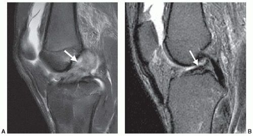Figure 2.1 A: Fat-suppressed, T2-weighted fast spin echo-XL (FSE-XL) image of a patient with acute anterior cruciate ligament (ACL) disruption (arrow) that demonstrates abnormal morphology (indistinct, discontinuous ligament fibers and mass effect) and abnormal increased signal intensity (due to intrasubstance hemorrhage and edema). B: Fat-suppressed, T2-weighted FSE-XL image of a patient with chronic ACL tear (arrow) with abnormal morphology (ligament discontinuity, attenuation, and laxity) but normal signal intensity.

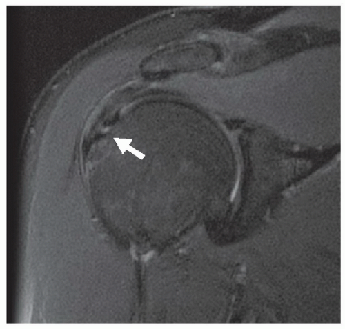Figure 2.2 Fat-suppressed, T2-weighted FSE-XL image of a patient with surgically confirmed, partial thickness, undersurface tear of the distal supraspinatus tendon (arrow). There is focal abnormal T2 signal at the tear site; however, the tendon morphology is grossly normal.

These cases present just a few examples of the application of basic interpretation techniques in analyzing musculoskeletal pathology. Multiple additional examples will be included throughout the remaining chapters of the text that more specifically deal with targeted anatomic locations.

TISSUE CHARACTERIZATION

The process of extracting information about tissue type and pathology by MR techniques has been called “tissue characterization.” This description has often been applied specifically to the use of quantitative measurements of relaxation times. Many studies of tissue characterization by in vivo measurement of relaxation times have appeared in the literature.¹^,²^,³^,⁴^,⁵^,⁶^,⁷^,⁸ These have generally not demonstrated a strong clinical role for “tissue characterization,” although it is fair to say that the hypothesis that accurate measurement of tissue relaxation times may be clinically useful has not yet been adequately tested.

Given the expanded definition for tissue characterization described above, what are the properties that are important in clinical imaging? A key word in this question is “imaging.” Some of the tissue properties that are important in this context are unique to the imaging process. This includes anatomic detail, which can demonstrate a lesion
solely by its effect on morphology (Fig. 2.7). Another similar property is tissue texture: Mass lesions in muscle are often characterized by their homogeneous texture, compared to the reticulated texture of normal muscle (Fig. 2.8).⁹ Even some of the classical tissue characterization parameters have special meanings in the imaging context.

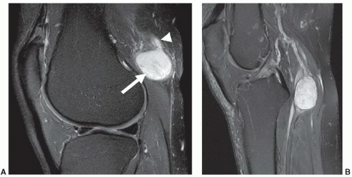Figure 2.3 A: Fat-suppressed, T2-weighted FSE-XL image of a patient with surgically confirmed peripheral nerve sheath tumor (PNST) of the tibial nerve within the upper popliteal fossa (arrow). The imaging morphology allows a confident imaging diagnosis, in this case demonstrating continuity with a traversing nerve structure (arrowhead). B: Fat-suppressed, T2-weighted FSE-XL image of a different patient with surgically confirmed PNST of the tibial nerve within the lower popliteal space with typical findings of a fusiform mass contiguous with the traversing nerve.

MR images basically reflect the distribution of mobile hydrogen nuclei. The brightness of each image pixel depends on, among other things, the density of mobile protons in the corresponding volume element and on the way that these protons respond to the externally superimposed static and fluctuating magnetic fields (see Chapter 1). This response depends on the chemical and biophysical environment of the protons and is described concisely by the relaxation times T1 and T2.

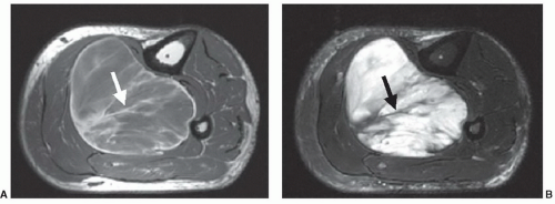Figure 2.4 Axial T1- (A) and T2-weighted (B) images of a surgically confirmed myxoid liposarcoma of the deep posterior compartment of the lower calf. Careful assessment of the internal architecture of the mass demonstrates linear, fatty strands that confirm the diagnosis (arrow). Most soft tissue sarcomas have a nonspecific MR appearance that does not allow a definitive diagnosis as in this case.

The spin-lattice relaxation time, T1, is an exponential time constant that describes the gradual increase in magnetization that takes place when a substance is placed in a strong magnetic field (Fig. 2.9). T1 predicts the time that it will take for nearly two-thirds (actually about 63%) of
the longitudinal magnetization to be restored after it has been tipped 90° by a radio frequency (RF) pulse. The spinlattice relaxation time of water protons in tissue depends in a complex fashion on rotational, vibrational, and translational motions and on the way that these are modified by proximity to macromolecules.

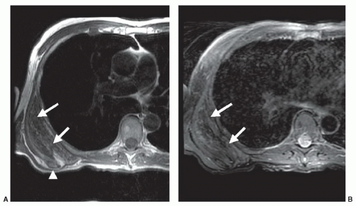Figure 2.5 Axial T1- (A) and T2-weighted (B) images of the upper torso demonstrate the typical location and appearance of an elastofibroma dorsi (arrows). The elliptical shaped, fibro-fatty mass is located deep to the serratus muscle and inferior margin of the scapula (arrowhead).

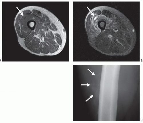Figure 2.6 Axial T1- (A) and T2-weighted (B) images of the thigh in an adult male patient with a palpable mass following incidental trauma. Study demonstrates an ill-defined region of reticulated and hazy abnormal increased T2 signal and mass effect in the vastus intermedius that contains an irregular central fluid collection (arrow). Corresponding AP radiograph (C) demonstrates faint, peripheral mineralization in a zonal pattern, which confirms the diagnosis of evolving myositis ossificans traumatica.

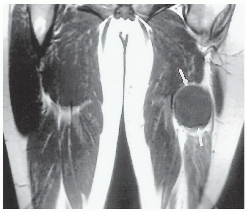Figure 2.7 Malignant soft tissue tumor (arrows), which is differentiated from adjacent muscle by its mass effect and homogeneity rather than by a signal intensity difference.

The spin-spin relaxation time, T2, is a time constant that describes the rate of exponential decay of transverse magnetization that would occur if the field was perfectly homogeneous (Fig. 2.10). Thus, for a spin-echo sequence, the net transverse magnetization at an echo delay time of TE = T2 will be approximately two-thirds (actually 63%) less than what was present immediately after the 90° pulse. The transverse magnetization is the component that creates a signal in MRI. Like T1, the spin-spin relaxation time depends on the natural motions of molecules. It is also affected by other processes that will be described later in this chapter.

It is difficult to accurately measure in vivo relaxation times with most MR imagers. These difficulties result from the necessity of irradiating a large but well-defined volume with RF energy and performing the steps required to create animage. Slice-selective 90° and 180° RFpulses, for instance, tend to be inaccurate near the boundaries of the section.¹⁰ The signal obtained from tissue that is irradiated with inaccurate RF pulses will not be the same as that obtained with ideal pulses. Relaxation times calculated from such measurements will be correspondingly incorrect. Other problems include the effects of applied field gradients, motion, and the small number of data points that are typically acquired.

In spite of these problems, properly performed in vivo relaxation time measurements are surprisingly reproducible with the same imager when they are performed on tissues that are stationary.¹¹^,¹² On the other hand, physiological motion can produce large random and systematic errors in relaxation times calculated from image data.¹³ Relaxation times obtained with one type of MR imager are usually not directly comparable to data obtained for the same tissue with another imager. This is because of the imager-specific systematic errors described above and the fact that relaxation times are field strength dependent. The T1 of muscle tissue, for instance, is nearly twice as long at 1.5 T (Tesla) as it is at 0.15 T.¹⁴^,¹⁵

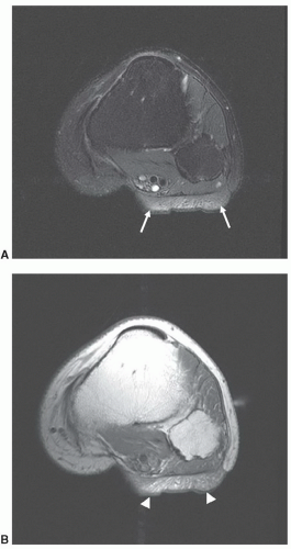Figure 2.8 A: A T2-weighted image of a patient who previously underwent surgical resection of a sarcoma from the anterior aspect of the leg demonstrates a mass with high signal intensity (arrow) that suggests tumor recurrence. B: A T1-weighted image of the same area demonstrates tiny streaks of fat (arrowheads) within the mass, typical of muscle, which effectively rules out tumor. The mass was a muscle flap that was placed in the tumor bed at the time of initial resection.

Given these problems, it is not surprising that clinical applications requiring quantitative measurement of tissue
relaxation times have been slow to emerge. Nevertheless, it is essential to understand the relative relaxation time relationships of tissues and pathological processes, because this is the key to understanding the highly variable gray scale of MRI.

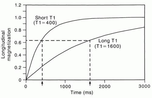Figure 2.9 The T1 relaxation time describes the regrowth of longitudinal magnetization after it is reduced to zero by a 90° RF pulse.

Spin density (mobile proton density, hydrogen density) is another important property that determines the appearance of tissue in magnetic resonance images. Few in vivo measurements of tissue spin density have been reported. This is probably because absolute measurements are difficult to perform with imagers. The derived spin densities are relative values that can only be compared within the same image. Nevertheless, spin density differences are an important source of image contrast in some tissues. There are large differences between the spin density of adipose tissue and muscle, for instance.¹⁶

Many other physical properties can potentially be measured or monitored by MR techniques to noninvasively characterize tissue. These include measuring the diffusion rate of water protons¹⁷^,¹⁸^,¹⁹^,²⁰ and differentiating between groups of protons on the basis of the characteristic chemical shift in their resonant frequency.³^,²¹^,²²^,²³^,²⁴^,²⁵^,²⁶^,²⁷^,²⁸^,²⁹^,³⁰^,³¹

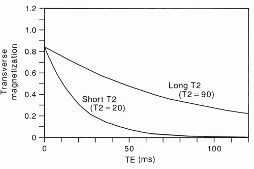Figure 2.10 The T2 relaxation time describes the exponential decay of magnetization in the transverse plane after it is placed there by a 90° RF pulse.

SIGNIFICANCE OF TISSUE RELAXATION TIMES

A detailed discussion of the physical mechanisms that determine relaxation time in biological systems is beyond the scope of this chapter. Indeed, these processes are as yet relatively poorly understood. Nevertheless, someof the concepts in the current view of this area are useful for understanding the appearance of normal and pathological tissue in clinical images.

Relaxation times describe the time course of the bulk magnetization of resonating protons following the application of perturbing RF pulses. The bulk magnetization is a vector quantity (i.e., having a magnitude and direction) that is the sum of the minute magnetic contributions of each of the resonating protons in tissue. The magnetic behavior of individual protons is quantum mechanical in nature, but the process of summing huge numbers of protons results in
a bulk magnetization vector that can assume a continuous range of magnitudes and orientations.

As already noted, the spin-lattice relaxation time (T1) describes the restoration of the longitudinal component of magnetization after it has been destroyed or reduced by an RF pulse. For this to happen, some of the protons that have been boosted into a higher energy level by the RF pulse must give up energy to the surrounding environment (sometimes called the “lattice”). This corresponds to reorienting individual proton magnetic moments from a direction that is roughly opposite to that of the main field to one that is, on average, in the same direction.

This process depends on interaction between the excited protons and neighboring nuclei in the lattice.³² The protons are subjected to a rapidly varying perturbation by the magnetic fields of adjacent nuclei. The frequency with which they vary is determined by the tumbling and translational motions of the protons and their neighbors. The perturbing motions are most effective for stimulating spin-lattice relaxation when they fluctuate at the Larmor frequency of the system.

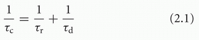
The characteristic length of time during which the magnetic field of a proton interacts with that of an adjacent nucleus with a magnetic moment is called the correlation time, τ.³² Essentially, this quantity is proportional to the period (i.e., inversely proportional to the frequency) of the cyclic field fluctuations caused by motion. Each mode of molecular motion has a characteristic correlation time. For tumbling motion, the correlation time is proportional to the period of rotation (Fig. 2.11). For translational motion, the correlation time can be regarded as proportional to the average time between the Brownian “jumps.” The combined correlation time is the parallel sum of the individual τ values associated with each of the perturbing motions:

As shown in Figure 2.12, the spin-lattice relaxation time decreases to a minimum as correlation time is lengthened, and then increases again. The position of the minimum of this curve is dependent on the Larmor frequency and, thus, the strength of the B₀ field.³³ Free water has a short correlation time of about 10^-12 seconds and thus it has a long spin-lattice relaxation time.

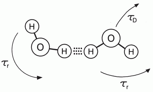Figure 2.11 As water molecules tumble and randomly jump in Brownian motion, the dipole moments of protons interact with a characteristic period that is called the correlation time.

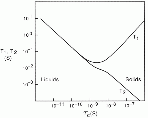Figure 2.12 Relationship between correlation time and the T1 and T2 relaxation times.

The spin-spin or T2 relaxation time of protons is also dependent on correlation times. It is also strongly affected by slowly varying and static magnetic fields at the molecular level.³² Such fields form gradients that cause moving protons to process at rates that have a small, random variation with time. Thus, they do not stay in phase with each other for as long as they would without the static field gradients, and this is reflected as a reduction in the T2 relaxation time (see Chapter 1). Figure 2.12 shows that in contrast to the T1 relaxation time, T2 continues to shorten as correlation times become longer and longer. Thus, the proton T1 and T2 relaxation times of solids, which have very slow molecular motion and longer correlation times, will be long and short respectively.

Although pure water has long T1 and T2 relaxation times of more than 2 seconds, much shorter relaxation times are typically observed in tissue. This is a result of the hydrophilic properties of many macromolecules. These molecules, which include proteins and polynucleic acids, have electric dipole and ionic sites that allow hydrogen bonding with water molecules in solution (Fig. 2.13).³⁴^,³⁵^,³⁶ The water in this hydration layer is less mobile than free water, and thus the correlation time is longer (τ_c = 10^-9 s). As a result, the T1 and T2 of hydration water are much shorter than that of free water.

The residence time of individual water molecules in the hydration layer of macromolecules is transient. Thus, individual water protons may alternately experience conditions that are favorable and unfavorable for relaxation as they exchange back and forth between bound and free states,
respectively. Under these “fast exchange” conditions, the observed relaxation time of water protons will be an average of the relaxation times in the bound and free states, weighted by the fraction in each state.³⁴

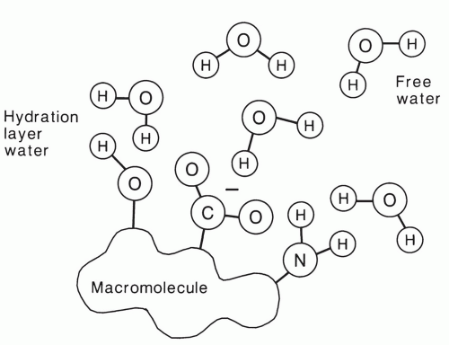Figure 2.13 Two-state model for organization of water in cytoplasm.

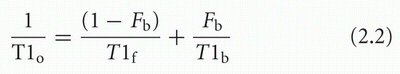
where T1_o is the observed T1, T1_f and T1_b are the relaxation times in the free and bound states, respectively, and F_b is the fraction of bound protons. The equation for T2 is similar. More complex models have been created to explain tissue relaxation behavior,¹⁴ but this simple, two-state, fast exchange model is very helpful for understanding clinical images. The T1 relaxation time of free water is approximately 2,500 ms, whereas that of hydration water is less than 100 ms. The model predicts that relaxation times of tissues with higher bound water fractions will be shorter than tissues that have a larger percentage of free water.

Tissue water proton relaxation times depend on many other factors. Field strength is one of the most important of these.¹⁴^,¹⁵^,³⁷^,³⁸ The trough of the T1 relaxation time curve in Figure 2.12 moves upward and to the left as field strength increases.³³ This means that the relaxation times of protons with correlation times in this range (bound water protons, for instance) will be longer at higher field strengths. It follows that the T1 relaxation time of most tissues increases with field strength because of the influence on the bound water component. In contrast, the T2 relaxation times of most tissues are relatively independent of field strength, except for a clinically important exception described below.

Paramagnetic contrast agents like Gd-DTPA can strongly affect tissue relaxation times when they are present.³⁹ These are substances with very strong magnetic moments that can enhance the relaxation of neighboring protons by perturbing them in a manner analogous to the way that proton fields interact with other protons. Many of these agents are paramagnetic by virtue of the presence of an unpaired orbital electron. The magnetic dipole moment generated by the unopposed electron is about 700 times stronger than the magnetic moment of a proton. The proton relaxation enhancement effect of these molecules is correspondingly intense.

When a sufficient amount of paramagnetic agent is added to an aqueous solution, the T1 and T2 relaxation times are shortened. The effect can be represented by the following equations:

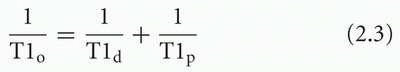
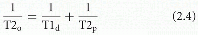
where T1_o and T2_o are the new observed relaxation times, T1_d and T2_d are the (diamagnetic) relaxation times of the solution or tissue without the paramagnetic agent, and T1_p and T2_p represent the extra relaxation process provided by the addition of the paramagnetic material. These latter quantities depend on the concentration of paramagnetic material:

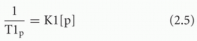
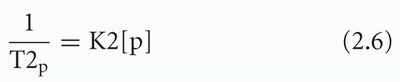
where [P] is the concentration of the paramagnetic material and K1 and K2 are constants that depend on the type of paramagnetic agent and on the characteristics of the tissue or solution.

Paramagnetic material may be endogenous in origin or it may be exogenously administered as a contrast agent for MRI. Endogenous paramagnetic materials are not believed to be present in sufficient concentration to affect the relaxation behavior of most normal human tissues significantly, but they do have a substantial effect in some pathological states such as transfusional hemosiderosis.⁴⁰

RELAXATION TIMES OF MUSCULOSKELETAL TISSUES

Tables of quantitative in vivo relaxation time measurements¹⁴ are of limited clinical usefulness because they are dependent on the field strength and on technical details of the imager and measurement method. Nevertheless, a general understanding of the relative relaxation characteristics of normal and pathological tissues is absolutely essential for competent interpretation of clinical magnetic resonance imagery. This task is relatively easy for the musculoskeletal system because the number of different tissues is small.

At the field strengths commonly used for proton imaging (0.15 T to 1.5 T), the T1 relaxation times of most soft tissues range between 250 and 1200 ms. The range of T2 values for most soft tissues is between approximately 25 and 120 ms.
Fluids and fibrous tissue depart from this range. The relative relaxation times of musculoskeletal tissues are summarized in Table 2.1.

Table 2.1 Relative Relaxation Times of Musculoskeletal Tissues

Tissue	T1	T2
Muscle	Medium	Short
Adipose tissue	Short	Medium
Nerve	Medium	Medium
Other soft tissue	Medium to long	Medium to long
Tendon, bone	—	Very short

These relationships can be summarized in a simple relaxation time map (Fig. 2.14). This figure shows that most musculoskeletal soft tissues fall into three distinct classes. Adipose tissue is characterized by its short T1 relaxation time in comparison to most other tissues, which dominates its appearance with most common MRI techniques. Healthy skeletal muscle has a short T2 relaxation time that is characteristic. Most other soft tissues, including tumors, have T1 relaxation times that are longer than that of adipose tissue and T2 relaxation times that are longer than that of muscle. The mobile proton density of bone, tendon, and dense fibrous tissue is low so that these tissues have low intensity in most MR images. These relationships form the basis for understanding and manipulating contrast in clinical MR of the musculoskeletal system.

EFFECT OF PATHOLOGY ON TISSUE RELAXATION TIMES

The relaxation times of many musculoskeletal tissues change in rather distinctive ways when they are affected by specific pathological processes.⁴¹ The significance and basic biophysical mechanisms for these changes are relatively poorly understood and few clinical applications have been demonstrated for their quantitative measurement. But they do result in diagnostically useful changes in the signal intensity and contrast of tissues in MR images. The general trend of the relaxation time changes for some important musculoskeletal disease processes is summarized in Table 2.2.

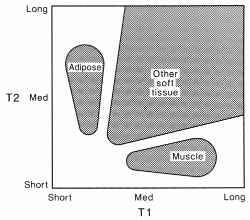Figure 2.14 Relaxation time map for musculoskeletal tissues.

Table 2.2 Relaxation Times for Common Musculoskeletal Disorders

Disease Process	T1	T2
Inflammation	Increased	Increased
Neoplasia	Increased	Increased
Fibrosis	—	Decreased
Fatty infiltration	Decreased	—
Interstitial hemorrhage	Increased	Increased

Inflammation

Inflammatory processes are generally characterized by prolongation of T1 and T2 relaxation times.⁴² The presence of edema seems to be the most likely mechanism to explain these changes. Accumulation of extracellular and possibly intracellular water causes an increase in the total water content of tissue. The previously described two-state, fast exchange model is helpful for understanding how even a small change in water content can result in a large alteration in relaxation times. Since water protons freely diffuse between the intracellular and extracellular spaces and the number of macromolecular binding sites is relatively fixed, the increased water content represents an increase in the fraction of free water.

Figure 2.15 shows theoretically expected tissue T1 values for various free water fractions, calculated using Eq. 2.2. The relaxation times T1_f and T1_b were assigned values of 2,500 and 50 ms, respectively. The resulting T1 relaxation time rapidly increases as the fraction of free water increases above
85%. Note, for instance that a 1% increase in free water from 91% to 92% causes a 10% increase in relaxation time.

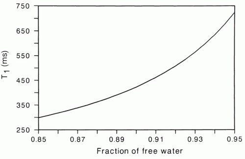Figure 2.15 Relationship between spin-lattice relaxation time and fraction of unbound or free water with a fast exchange, two-state model for tissue relaxation times.

Neoplasms

With certain exceptions, most solid neoplasms are characterized by relaxation times that are prolonged relative to their host tissues. Many studies of this phenomenon have appeared in the literature.⁴³

Only gold members can continue reading. Log In or Register to continue