Variable
Normal values
Abnormal values
CAM location
Lesion between 12 and 4 o’clock
Alpha angle
>42°
Coronal center-edge angle
41°
<20°
Sagittal center-edge angle
31°
<20°
Neck-shaft angle
126–139°
Coxa vara <126°
Coxa valga >139°
Acetabular version 1 o’clock
5°
Acetabular version 2 o’clock
10°
Acetabular version 3 o’clock
15°
>30°
Femoral version angle
15–20°
>30°
McKibbin index
30–60°
>60 or <30°
AIIS width
1 cm
Distal base of AIIS to acetabular rim
≥0.5 cm
<0.5 cm
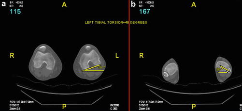
Fig. 1
Tibial version is measured by finding the angle between the line along the posterior contour of the proximal tibia (a) and the intermalleolar axis (b). Normal tibial version angle ranges between 18° and 47° in skeletally mature adults
Radiation Exposure
Radiation dose is measured in units of rem or sievert (Sv), where 100 rem is equivalent to 1 Sv. A single chest radiograph exposes the patient to approximately 0.02 mSv, while a CT scan of the pelvis exposes the patient to approximately 3–4 mSv [3]. This amount of exposure is significant in light of prior evidence demonstrating an increase in cancer risk with radiation doses in excess of 50 mSv [4]. New image reconstruction techniques, such as adaptive statistical iterative reconstruction (ASiR), have made it possible to reduce the radiation dose to patients up to 50 % [5, 6]. Several dose reduction strategies exist to achieve diagnostic image quality while minimizing patient radiation exposure. For routine contrast-enhanced CT of the pelvis , the CT protocol can be tailored based on patient size and clinical indications by modifying the maximum tube current (mA) and noise index (NI), which can generally be increased with increasing patient size [7]. The lower tube potential (kV) can also be adjusted based on patient size [8]. ASiR has demonstrated not only significant radiation reduction but also improved image quality in comparison with traditional filtered back-projection techniques [7, 8]. CT protocols can be customized in order to lower radiation doses particularly for pregnant or pediatric patients without compromising image quality.
Pathological Entities
Femoroacetabular Impingement (FAI)
Cam, pincer, and mixed types of impingement can occur between the proximal femur and the acetabulum. Cam-type FAI occurs when a nonspherical femoral head leads to an abnormal contour of the head-neck junction. This morphologic abnormality can impinge with the acetabulum and labrum when the hip is placed in positions of flexion, adduction, and internal rotation. Cam-type impingement may result from a variety of causes including distortion of the physis during growth, Legg-Calvé-Perthes syndrome, previous trauma, or slipped capital femoral epiphysis.
Preoperative planning with a 3D CT protocol can help tailor the operative approach (Table 1). Cam lesion location is commonly defined by using clockface terminology. Typically, 12 o’clock represents the most superolateral aspect, 3 o’clock represents the most anterior aspect, and 6 o’clock represents the most inferomedial aspect of the femoral head-neck junction. The cam is most commonly found between 12 o’clock and 4 o’clock [9]. Cam lesions that are beyond 12 o’clock (i.e., 11 o’clock) toward the posterior aspect of the hip are difficult to address arthroscopically and may be more amenable to an open procedure.
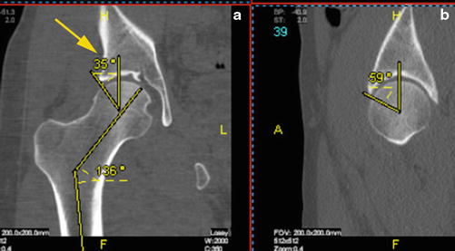
An objective method to quantify the size of the cam lesion is the alpha angle. The alpha angle is measured at the maximal offset where the abnormal bony contour of the femoral head-neck junction extends beyond the spherical confines of the femoral head. Using CT, the alpha angle can be measured on multiple planes. The measurement is an angle from the axis of the femoral neck to the point where the head-neck junction loses its spherical contour [10] (Fig. 2). An alpha angle greater than 42° is considered abnormal [10]. In a retrospective, comparative study, Hetsroni et al. found that the alpha angles for men and women presenting with hip pain and labral tears were 63.6 ± 10.8° and 47.8 ± 9.5°, respectively [11].
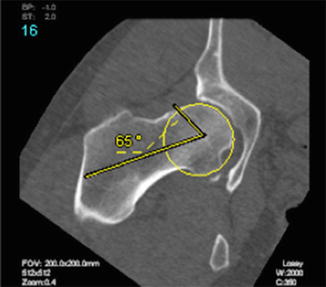
Fig. 2
Coronal oblique view alpha angle determined by measuring the angle subtended between a line along the axis of the femoral neck and the point at which the femoral head loses its sphericity at its maximal deformity. The alpha angle and cam location in this case are 65° and between 1 and 3 o’clock, respectively. Note that the alpha angle can be measured from the coronal, sagittal, and radial views. An angle > 42° is considered to be abnormal
The neck-shaft angle (NSA) is measured on the coronal view. This NSA angle is the angle subtended by the femoral neck and diaphyseal axes (Fig. 3). The neck axis is defined by the line connecting the center of the femoral head and the center of the femoral neck at its isthmus. The diaphyseal axis is defined by the line connecting the midpoint of two lines drawn perpendicularly across the diaphysis of the femur. A normal NSA is between 126° and 139°. Coxa vara is defined as a NSA <126° and is more consistent with impingement. Coxa valga is defined as NSA >139° and is more consistent with instability and dysplasia [12].
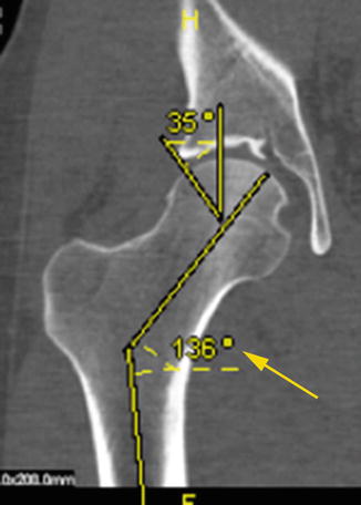
Fig. 3
Neck-shaft angle (arrow) is normally between 126° and 139°
Pincer-type FAI occurs when the abnormal morphology is in the acetabulum. Several possible causes of abnormal acetabular morphology include coxa profunda, protrusio, rim prominence, and retroversion. Acetabular version angle is formed by the intersection of the line perpendicular to the line between the posterior pelvic margins and the line connecting the anterior and posterior rim of the acetabulum (Fig. 4) [13]. This measurement is conducted at 1 o’clock, 2 o’clock, and 3 o’clock with normal being approximately 5°, 10°, and 15°, respectively. Patients with retroverted acetabulums are associated with pincer-type FAI.
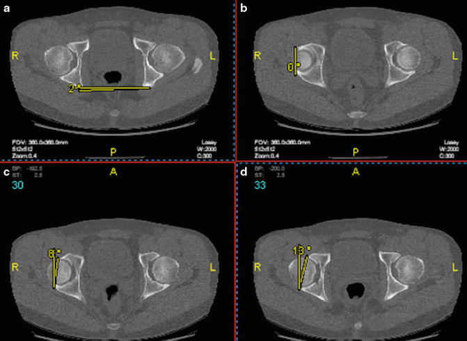
Fig. 4
Acetabular version. (a) The angle created from the line connecting the posterior pelvic margin and horizontal line of the image screen represents the amount of correction (2°) that will need to be added to subsequent measurements in B, C, and D. (b) Acetabular version at 1 o’clock measuring 2° (0° + 2° of correction). (c) Acetabular version at 2 o’clock measuring 10° (8° + 2° of correction). (d) Acetabular version at 3 o’clock measuring 15° (13° + 2° of correction). Acetabular version angle is normally 5°, 10°, and 15° at 1 o’clock, 2 o’clock, and 3 o’clock, respectively
Subspine Impingement
Subspine impingement occurs when there is direct impingement of the inferior femoral neck along with the labrum, capsule, and indirect head of the rectus femoris against the anterior inferior iliac spine (AIIS). This type of impingement occurs in positions of straight hip flexion. AIIS morphology can be typed and subtyped based on the direction of slope of the AIIS as well as the presence or absence of a clear subspine space (Figs. 5 and 6) (Tables 2 and 3). AIIS type I has an upsloping morphology, which does not contribute to impingement. AIIS type III has a downsloping (crossing the rim) morphology that is more likely to cause impingement. AIIS subtype A has a clear subspine space, which does not contribute to impingement. However, AIIS subtype B has a subspine bone prominence or rim level-based AIIS that is more likely to cause impingement. Therefore, AIIS types II and III and subtype B have a higher predilection for subspine impingement [14]. The AIIS is also assessed to determine the degree of subspine impingement. The distance from the distal base of the AIIS to the acetabular rim should be ≥0.5 cm. A measurement of <0.5 cm is consistent with subspine impingement. The width of the AIIS should be about 1 cm.
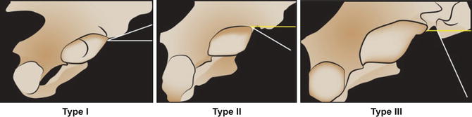
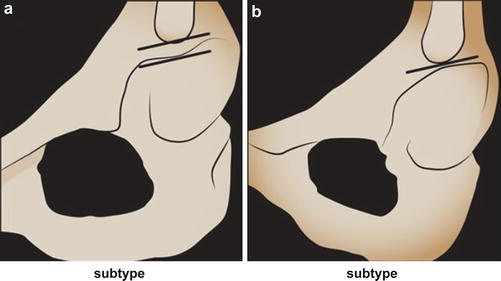
Fig. 5
AIIS morphology types. Type I with an upsloping AIIS morphology. Type II with a flat or downsloping AIIS morphology. Type III with a significantly downsloping AIIS morphology
Fig. 6
AIIS morphology subtypes. Subtype A with a subspine clear space. Subtype B with a subspine bone prominence or rim level-based AIIS
Table 2
AIIS morphology
Type | Description | CT definitions | Clinical importance |
|---|---|---|---|
I | Upsloping | Upsloping on Ischium view | AIIS does not contribute to impingement |
II | Flat to downsloping | Flat to downsloping on ischium view, but does not cross the rim | AIIS may contribute to impingement |
III | Significant downsloping | Downsloping and crosses the rim | AIIS may contribute to impingement |
Table 3
AIIS Subtype Morphology
Subtype | Description | CT Definitions | Clinical Importance |
|---|---|---|---|
A | Clear subspine space | No secondary extension to rim | AIIS does not contribute to impingement |
B | Subspine bone prominence, or rim level-based AIIS | Caudal extension of AIIS on ilium wall to acetabular rim level | AIIS may contribute to impingement |
Acetabular Dysplasia
Acetabular dysplasia is defined as an abnormality with the version, volume, or inclination of the acetabulum [15]. The morphologic deformity places a greater concentration of weight-bearing forces on a smaller area of articular cartilage, resulting in degenerative soft tissue injuries and osteoarthritic symptoms. Patients with subtle dysplasia are difficult to identify, particularly as a spectrum of disease involve both dysplasia and FAI, which often have overlapping symptoms [16]. Morphologically, acetabular dysplasia is one of the most complex 3D deformities. CT reconstruction circumvents the limitations of traditional 2D radiographic screening, allowing for more accurate estimations of the severity of dysplasia. Measurements such as center-edge angle (CEA), acetabular index (AI), and acetabular sourcil angles can be used to evaluate for dysplasia.
The CEA corresponds to the degree of coverage of the femoral head by the acetabulum. A higher CEA indicates a greater degree of coverage, whereas a lower CEA indicates a lesser degree of coverage. The center-edge angle can be measured on the sagittal or coronal views. The specific cuts chosen to measure these angles are through the center of the femoral head. The coronal CEA is measured by first drawing a line through the center of the femoral head perpendicular to the transverse pelvic axis. Next, a line is drawn through the center of the femoral head to the superolateral aspect of the acetabular roof. The angle between these lines defines the coronal CEA (Fig. 7a). This corresponds to the lateral CEA on radiographs [17], where a CEA <20° is considered to be dysplastic [18]. The average CEA is approximately 41° [19]. The sagittal CEA is measured by first drawing a vertical line through the center of the femoral head. Next, a line is drawn through the center of the femoral head to the most anterior aspect of the acetabular rim. The angle between these lines defines the sagittal CEA (Fig. 7b). This corresponds to the anterior CEA on radiographs where an anterior CEA <20° is considered to be dysplastic [20]. The average anterior CEA angle is approximately 31° [19]. In patients with a CEA <20°, a procedure such as a periacetabular osteotomy (PAO) may be indicated.
 Neuromuscular Hip Disorders: Focus on Cerebral Palsy
 Femoral Deformities: Varus, Valgus, Retroversion, and Anteversion
 Rehabilitation of Non-Operative Hip Conditions
 Surgical Technique: Open Proximal Hamstring Repair
 Subspine Impingement and Surgical Technique
 Atraumatic Instability and Surgical Technique


Related posts:
Neuromuscular Hip Disorders: Focus on Cerebral Palsy
Femoral Deformities: Varus, Valgus, Retroversion, and Anteversion
Rehabilitation of Non-Operative Hip Conditions
Surgical Technique: Open Proximal Hamstring Repair
Subspine Impingement and Surgical Technique
Atraumatic Instability and Surgical Technique
Stay updated, free articles. Join our Telegram channel
Full access? Get Clinical Tree
