Basic Principles and Terminology of Magnetic Resonance Imaging
Robert A. Pooley
Joel P. Felmlee
Richard L. Morin
This chapter is presented to acquaint those new to magnetic resonance imaging (MRI) with the fundamental concepts and basic principles responsible for the nuclear magnetic resonance (NMR) phenomenon and MRI. At the outset, it is important to understand that this chapter is intended to be tutorial in nature. In addition to the fundamental concepts of the physical phenomenon of NMR itself, techniques relevant to clinical imaging are discussed in the context of a tutorial presentation of fundamentals for those new to MRI. It is important to appreciate that the physics principles associated with MRI often take a while to assimilate. There are many approaches to the discussion and presentation of the fundamental physics of MRI. Technical details and in-depth coverage can be found in MRI texts and review articles.1,2,3,4,5 The appendix lists terms that have been selected from the American College of Radiology glossary of MR terms6 and are provided for the sake of completeness and reference.
A chronology of the historical development of MRI is listed in Table 1.1. The principle of NMR was first elucidated in the late 1940s by Professor Bloch at Stanford and Professor Purcell at Harvard. In 1952, they shared the Nobel Prize in physics for their work. The importance of this technique lies in the ability to define and study the molecular structure of the sample under investigation. In the 1970s, the principle of NMR was utilized to generate cross-sectional images similar in format to X-ray computed tomography (CT). By 1981, clinical research was underway.
The intense enthusiasm and the rapid introduction of MRI into the clinical environment stem from the abundance of diagnostic information present in MR images. Although the image format is similar to that of CT, the fundamental principles are quite different; in fact, an entirely different part of the atom is responsible for the image formation. In MRI it is the nucleus that provides the signal used in generating an image. We note that this differs from conventional diagnostic radiology in which the electrons are responsible for the imaging signal. Furthermore, it is not only the nucleus of the atom but also its structural and biochemical environments that influence the signal.
Currently, fast imaging techniques are increasing as important clinical methods. Echo planar imaging (EPI), as well as fast spin echo and gradient echo based acquisitions, allows image acquisition in the sub-second to breath hold (15 second) range. These techniques hold the potential for high-resolution studies acquired quickly, thereby “freezing” many physiologic motions. Using these fast acquisition techniques, encoding functional and flow information into the image are areas of clinical interest and research.
Throughout this discussion we illustrate the underlying physics principles with analogies and discuss the nature of the physics from a “classical” rather than a “quantum mechanical” point of view. Both approaches result in accurate explanations of the NMR phenomenon; however, they differ in their mathematical constructs and visualization of the underlying physical principles.
THE NUCLEAR MAGNETIC RESONANCE EXPERIMENT
When certain nuclei (those with an odd number of protons, an odd number of neutrons, or an odd number of both) are placed in a strong magnetic field, they align themselves with the magnetic field and begin to rotate at a precise rate or frequency (Larmor frequency). If a radio transmission is made at this precise frequency, the nuclei will absorb the radio frequency (RF) energy and become “excited.” After termination of the radio transmission, the nuclei will calm down
(or relax) with the emission of radio waves. The emission of RF energy as the nuclei relax is the source of the NMR signal. The ability of a system to absorb energy that is “packaged” in a particular kind of way is termed resonance. This condition is analogous to the pushing of a child on a swing. If the child is pushed at the highest point of return, then the maximum amount of energy is transmitted to the swing. Attempting to push the child at the midpoint of return results in a low transfer of energy, and in this sense would be off-resonance. Hence, the resonance condition in this case is the timing of pusheswith the exact frequency of the pendulum movement of the swing.
(or relax) with the emission of radio waves. The emission of RF energy as the nuclei relax is the source of the NMR signal. The ability of a system to absorb energy that is “packaged” in a particular kind of way is termed resonance. This condition is analogous to the pushing of a child on a swing. If the child is pushed at the highest point of return, then the maximum amount of energy is transmitted to the swing. Attempting to push the child at the midpoint of return results in a low transfer of energy, and in this sense would be off-resonance. Hence, the resonance condition in this case is the timing of pusheswith the exact frequency of the pendulum movement of the swing.
Table 1.1 Historical Development of MRI | ||||||||||||||||||||
|---|---|---|---|---|---|---|---|---|---|---|---|---|---|---|---|---|---|---|---|---|
|
The precession of nuclei about a magnetic field is similar in concept to the precession of a spinning top in the presence of a gravitational field, as illustrated in Figure 1.1. This type of rotation occurs whenever a spinning motion interacts with another force. Nuclei with an odd number of protons or neutrons or both possess a property of “spin,” which in this case interacts with the magnetic field, thereby inducing precession of the nuclei about the magnetic field. The precessional or Larmor frequency is determined by the individual nuclei and the magnetic field strength [given in the SI unit Tesla (T) or the centimeter-gram-second (cgs) unit gauss (G), where 1T = 10,000 G]. The mathematical definition of the Larmor frequency is given by
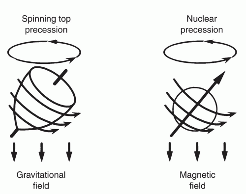 Figure 1.1 Illustration of precession. (Adapted from Fullerton GD. Basic concepts for nuclear magnetic resonance imaging. Magn Reson Imaging. 1982;1:39-55, with permission.) |
Table 1.2 Larmor (Resonance) Frequencies for Hydrogen | ||||||||||||||||
|---|---|---|---|---|---|---|---|---|---|---|---|---|---|---|---|---|
|
ω = γB0,
where ω is the Larmor frequency, B0 is the static magnetic field strength, and γ is the gyromagnetic ratio (a constant that is different for each nucleus). Larmor frequencies for various nuclei and field strengths are given in Tables 1.2 and 1.3. For protons at a field strength of 1.5T, the Larmor frequency is 64 megahertz (MHz), which is the same frequency used for transmitting the television signal of channel 3.
In summary, the fundamentals of the NMR experiment are illustrated in Figure 1.2 and consist of three steps: (a) placing a sample in a magnetic field, thereby inducing a nuclear precession, (b) transmitting an RF pulse at the Larmor frequency, and (c) “listening” for the returning NMR signal. Note that the frequency of the transmitted RF and the returning signal are dependent upon both the nuclei of interest and the magnetic field strength B0.
THE NUCLEAR MAGNETIC RESONANCE SIGNAL
The form of the RF signal produced by the NMR experiment depends on the number of nuclei present (spin density) and the time it takes for the nuclei to relax (T1 and T2). The parameter T1 (spin-lattice relaxation time) measures the rate of return of the nuclei to alignment with the static magnetic field (B0) and reflects the chemical environment of the proton. T2 (spin-spin relaxation time) measures the dephasing of the nuclei in the transverse plane and reflects the relationship of the proton to the surrounding nuclei.
Table 1.3 Larmor (Resonance) Frequencies AT 1.0 Tesla | ||||||||||||
|---|---|---|---|---|---|---|---|---|---|---|---|---|
| ||||||||||||
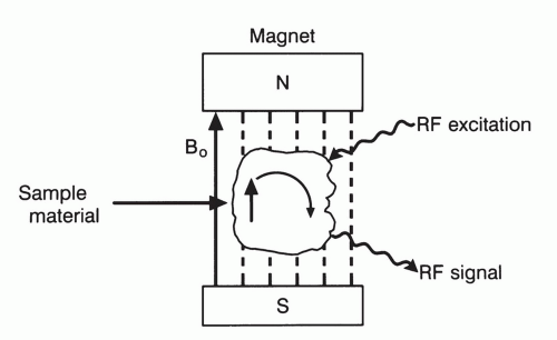 Figure 1.2 Basics of NMR measurements. Here the magnetization is nutated 90° by the RF excitation. (Adapted from Fullerton GD. Basic concepts for nuclear magnetic resonance imaging. Magn Reson Imaging. 1982;1:39-55, with permission.) |
These processes are illustrated in Figure 1.3. The degree to which the NMR signal depends on spin density, T1 or T2, is determined by the pulse sequence, which we shall discuss later. The nature of this signal and its decay due to relaxation are of fundamental importance and we shall discuss this process in detail.
The form of the basic NMR signal [free induction decay (FID)] is shown in Figure 1.4. The signal is a time oscillating waveform that is detected in the x-y or transverse plane, defined by the coordinate system for the experiment as shown in Figure 1.5. Note that after a 90° rotation, the magnetization vector is in the “transverse” plane. The received signal is oscillating because we measure it from the transverse plane as the magnetization vector rotates about the longitudinal axis. Hence, a rotating signal is translated into a sinusoidal time-varying voltage.
It is important to understand that we can only measure the macroscopic magnetization vector, that is, the algebraic summation of all nuclear spins under investigation (Fig. 1.6). In reality, not all nuclear spins in a sample precess at the same frequency. Each individual nucleus is influenced by a slightly different magnetic field due to the interactions of electrons that surround individual nuclei or the movements of adjacent molecules. The first process that occurs upon RF transmission is the phasing of individual nuclear spins to create the macroscopic magnetization vector Mxy (similar to the military command “fall in” given to a group of soldiers). This ensemble of phased nuclear spins then changes their orientation with regard to the z-axis. The rotation of this phased macroscopic magnetic vector is the property that we detect causing an oscillatory MR signal with time.
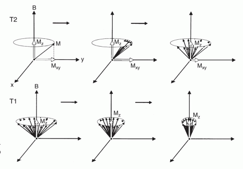 Figure 1.3 Diagram of T2 (spin-spin, transverse) relaxation and T1 (spin-lattice, longitudinal) relaxation after a 90° nutation pulse. |
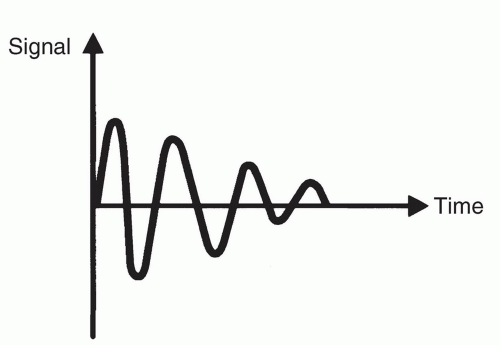 Figure 1.4 Plot of free induction decay (FID), the basic NMR signal. |
The decay of the signal as shown in Figure 1.4 occurs because following cessation of the RF transmission, the nuclear spins dephase. Since magnetization is a vector quantity, dephasing causes the macroscopic magnetic vector to decrease in magnitude. Since this activity takes place in the x-y or transverse plane, this process is also called transverse relaxation. In a chemical sense, this relaxation is due to interactions that occur between adjacent nuclei and is therefore termed spin-spin relaxation. The effect of T2
relaxation for substances with different T2 values is illustrated in Figure 1.7.
relaxation for substances with different T2 values is illustrated in Figure 1.7.
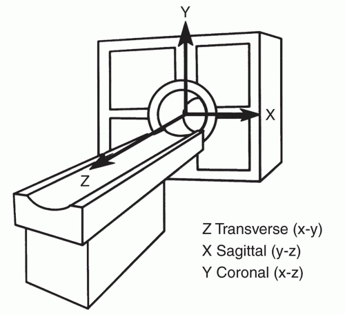 Figure 1.5 MRI coordinate system. |
As the above-mentioned dephasing or T2 relaxation occurs, the entire ensemble of nuclei return to alignment with the main magnetic field B0, which is oriented along the z-axis. Hence, the longitudinal or z component of the macroscopic magnetic vector “grows” or increases with time, as the protons realign with B0 and return to an equilibrium value. Since this T1 recovery occurs along the direction of the longitudinal axis, it is termed longitudinal relaxation. In a chemical sense, this process is governed by the strength with which an individual nucleus is bound to its chemical backbone (water, lipid, protein, etc.) and hence this process is often termed spin-lattice relaxation. The effect of T1 relaxation is represented in Figure 1.8 for substances of different T1 values.
MAGNETIC RESONANCE IMAGING
An illustration of an MRI system is shown in Figure 1.9. To conduct the NMR experiment, a strong magnet, radio transmitter, and radio receiver are necessary. To produce MR images, additional magnetic coils (gradient coils) are necessary to encode the signal and thus allow its origin to be determined. In addition, a computer system is necessary to control the sequencing of the RF, gradients, data collection, operations, and perform the final image reconstruction.
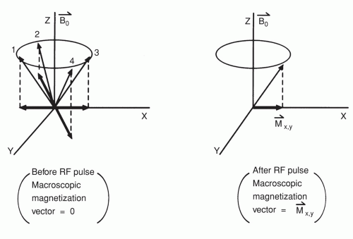 Figure 1.6 Illustration of the macroscopic magnetic vector formed by individual nuclei. A: Individual nuclei 1, 2, 3, and 4 precessing about the magnetic field B0. The measured macroscopic magnetization vector is zero due to the algebraic summation of x and y components of the randomly oriented nuclei. B: Macroscopic magnetization vector formed by the phasing of individual nuclei 1, 2, 3, and 4. The macroscopic magnetization vector measured is the component in the transverse plane, that is, Mx,y. |
 Figure 1.7 Plot of the loss of magnetization in the transverse (xy) plane following cessation of RF transmission. |
In the most common type of MRI, spatial localization is obtained using additional magnetic fields superimposed on the main magnetic field. The key to understanding this phenomenon lies in the Larmor equation. Recall that the precessional frequency is directly related to magnetic field strength. If a spatially varying magnetic field is superimposed on the main magnetic field, then precessional frequencies will be related to a location in space, analogous to the frequency obtained by the specific location of keys on a piano. This translation between frequency and spatial location is shown in Figure 1.10.
The most common imaging technique [two-dimensional Fourier transform or (2DFT)]7,8,9 involves the use of three such gradient fields to localize a point in space. It is important to understand that all three gradients will be turned on and off at different times. The particular application and relative timing of the x, y, and z gradients determine which axis (x, y, or z) is being localized. In general, signals will be localized by selective application of
slice selection, phase encoding, and frequency encoding gradients. A schematic diagram of the timing of these gradients is given in Figure 1.11. We describe each in detail for the acquisition of a transverse slice.
slice selection, phase encoding, and frequency encoding gradients. A schematic diagram of the timing of these gradients is given in Figure 1.11. We describe each in detail for the acquisition of a transverse slice.
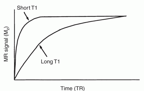 Figure 1.8 Plot of recovery of magnetization in the longitudinal (z) direction. |
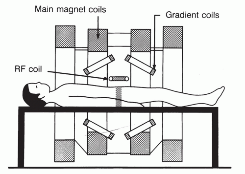 Figure 1.9 Diagram of MRI system. ((Adapted from Fullerton GD. Basic concepts for nuclear magnetic resonance imaging. Magn Reson Imaging. 1982;1:39-55, with permission.) |
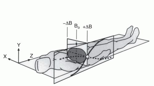 Figure 1.10 Diagram of spatial encoding of MR signal by superposition of magnetic field gradients (different resonance frequencies correspond to different positions along the gradient). |
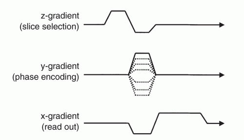 Figure 1.11 Gradient activation versus time for MRI acquisition of a single transverse slice. For this case, slice selection is in the craniocaudal (C-C) direction, phase encoding in the anteroposterior (A-P) direction, and frequency encoding in the right-left (R-L) direction. |
The slice is first selected by applying a gradient along the z-axis while applying an RF pulse with a narrow frequency range. This excites the nuclei only in the slice of interest so that they are all precessing at the same frequency and phase (Fig. 1.10). However, the signal we detect is from the entire slice, so at this point it is not possible to form an image.
Next, the relative phase of spin precession is modified by applying a gradient in the y-direction. This gradient causes the atoms at different location along y to precess at different frequencies while the y gradient is applied (Fig. 1.12). If no gradient is present, the nuclei precess at the Larmor frequency corresponding to the main magnetic field strength. If a slightly higher magnetic field is superimposed with a gradient as shown in Figure 1.12, the nuclei in row 1 precess at a slightly higher frequency than those in row 2; likewise for rows 2 and 3. When the gradient is turned off, all the rows will once again precess at the same frequency. However, since row1waspreviouslyprecessing at a slightly higher frequency than row 2, all the nuclei in row 1 will be slightly ahead of those in row 2; that is, they will be precessing at the same frequency but at different phases. Likewise, each successive row will precess at the same frequency but at a slightly different phase. To obtain discrimination in the phase encoding direction, this process must be repeated many (e.g., 256) times. This result of increased phase encoding for a coronal image with phase encoding in the superoinferior direction is shown pictorially in Figure 1.13.10
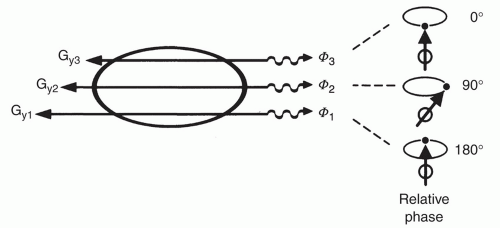 Figure 1.12 Phase encoding in the y-direction. Here the gradient increases from top to bottom. |
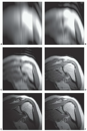 Figure 1.13 MRI phase encoding (10). All images are from the same acquisition (TR = 500, TE = 20, 2 excitation, 5 mm slice, 256 phase encoding steps). The original raw data were truncated to demonstrate the effect of phase encoding. A: 2 steps. B: 8 steps. C: 16 steps. D: 32 steps. E: 64 steps. F: 256 steps. |
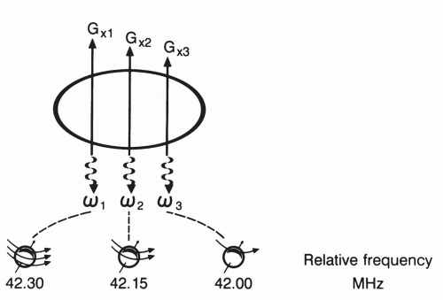 Figure 1.14 Frequency encoding in the x-direction. Here the gradient decreases from left to right. |
The precessing nuclei are frequency encoded by the application of a magnetic gradient in the x-direction. This gradient causes the atoms to precess at different frequencies (Fig. 1.14) and is usually applied while the MR signal is being collected (hence, it is sometimes called the readout gradient).
The MR signal is digitized and stored on the acquisition workstation (in “k-space”) for subsequent Fourier reconstruction to form the clinical image. Each point in k-space represents a different spatial frequency in the object being imaged. The strength of the MR signal (and thus the value of a data point in k-space) indicates the degree to which that spatial frequency is represented in the object. Lower spatial frequencies are located near the center of k-space and contain information related to image contrast. Higher spatial frequencies are located at the periphery of k-space and contain information related to image sharpness. This is demonstrated in Figure 1.15 by viewing k-space and the clinical images reconstructed from the center or periphery of k-space.
MAGNETIC RESONANCE IMAGING PULSE SEQUENCES
MRI pulse sequences are basically the recipe for the application of RF pulses, the sequencing of gradient pulses in the x, y, and z direction, and the acquisition of the resultant MR signal.
The most basic component of a pulse sequence is the specification of the RF excitation and subsequent signal detection. Timing diagrams for two pulse sequences [inversion recovery (IR) and spin echo (SE)] are given in Figures 1.16 and 1.17. Each sequence is discussed in detail.
The schematic diagram for the IR pulse sequence is shown in Figure 1.16. This sequence is characterized by the application of an RF pulse of sufficient power to tip the nuclei through 180°, an inversion time (TI), and the subsequent application of a 90° pulse (to rotate the magnetization into the transverse plane), followed by signal detection. This pulse sequence can be used to measure the longitudinal recovery of magnetization (Fig. 1.18). Because the range of measured magnetization for this pulse sequence varies from −Mz to + Mz, if phase-sensitive image reconstruction is employed, the magnitude of measured differences for a sample due to T1 relaxation may be larger with the IR sequence than those with the spin-echo technique below (in which the longitudinal magnetization varies from 0 to +Mz). These differences may not be as pronounced with magnitude reconstruction (Fig. 1.18). Hence, image contrast due to T1 differences can be greater with IR. Examples of images acquired using this pulse sequence and magnitude reconstruction are shown in Figure 1.19.
The pulse diagram for the SE pulse sequence is shown in Figure 1.17. The spin-echo pulse sequence is characterized by the application of a 90° pulse, which therefore tips the nuclei into the transverse or x-y plane. This is followed by successive 180° pulses, separated by the delay period TE, which causes the formation of successive signals for detection, which are termed spin echoes. The entire pulse sequence is repeated following the delay interval TR. The formation of spin echoes is demonstrated in Figure 1.20. The fundamental characteristic of this sequence lies in the fact that the nuclei dephase following the 90° pulse. If this dephasing spin system is rotated through 180°, individual spins will now travel toward one another instead of away from one another. When all spins meet one another, a spin echo is produced. Following that moment in time, the spin system will once again dephase and can be refocused or rephased with another 180° pulse. Depending upon the acquisition TE and TR, this sequence can be useful in demonstrating differences due to either T1 or T2 relaxation time as shown in Figure 1.21. Examples of images acquired using this pulse sequence are given in Figure 1.22. In summary, the spin density, T1, and T2 represent inherent properties of tissues. TE and TR are properties of the image acquisition that are under operator control. The TE and TR of an image acquisition can be manipulated such that the difference between signals from tissues (which ultimately determines the image contrast) is weighted by tissue spin density, T1, or T2 relaxation.
The previous discussion dealt with pulse sequences that were concerned only with RF excitation and signal detection. Hence, this discussion would be germane to spectroscopy as well as imaging. For MRI, the pulse sequence must also identify the timing information associated with the gradients necessary to prepare or localize the signal for image reconstruction.
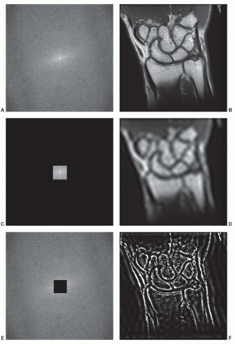 Figure 1.15 Reconstruction of k-space. A: Original k-space data. B: Image data reconstructed from A, showing good image contrast and spatial resolution. C: Center portion of k-space. D: Image data reconstructed from C, showing good image contrast but poor spatial resolution. E: Peripheral portion of k-space. F: Image data reconstructed from E, showing poor image contrast but good spatial resolution (edges). |
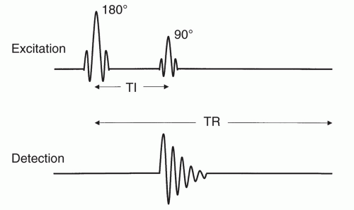 Figure 1.16 Inversion recovery pulse sequence. |
An example of an MRI pulse sequence is shown in Figures 1.11 and 1.23. We note that the gradients are labeled as slice selection, phase encoding, and readout (or frequency encoding). The reason for this specification is that slice selection can be along the transverse, coronal, or sagittal planes with phase and readout gradients along the other two orthogonal planes. The dotted lines indicating progression of phase encoding implies that this pulse sequence will be repeated many times with a differing amount of phase encoding at each repetition. The rest of the sequence (RF, Gx, Gz) will remain exactly the same with each repetition.
It is the variation in timing and relative temporal placements of the three magnetic gradient sequences that are largely responsible for the plethora of the imaging sequences currently available. We use such diagrams in later sections to understand the differences and consequences of employing various pulse sequences. An understanding of the effects of frequency shifts and dephasing effects are of central importance to understanding image characteristics and artifacts in MRI. Because this is a currently active area of development, similar techniques have been developed by different sources, resulting in different acronyms for essentially the same procedure.
It is important to note that although essentially similar results have been accomplished by various investigational groups and vendors, hardware and software differences in the exact realization may result in subtle but sometimes important image variation. Tables 1.4 and 1.5 present a compilation of the acronyms for similar imaging techniques.11,12 These acronyms represent in some cases broad classifications provided by various manufacturers, yet they are routinely used in the literature. For more information about any of these techniques, the reader is referred to the technical representatives of the particular vendor of interest.
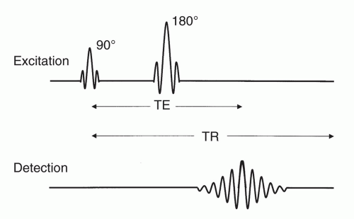 Figure 1.17 Spin-echo pulse sequence. |
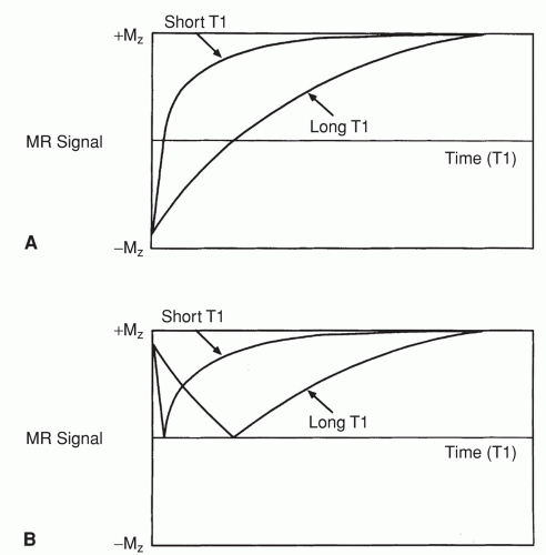 Figure 1.18 Recovery of magnetization for inversion recovery pulse sequence. A: Phase sensitive image reconstruction. B: Magnitude image reconstruction. |
MOTION EFFECTS
Motion artifacts can cause a range of degradation, depending upon the severity and the timing of the motion during the acquisition. The images in Figures 1.24 show how motion can reduce the image resolution, while not causing significant image ghosting. The wrist image in Figure 1.24A shows significant resolution loss when compared to the image in Figure 1.24B without motion. An important aspect of the image acquisition is the preparation of the patient to reduce motion; the part of interest must be adequately padded and supported well beyond the region of clinical interest, then immobilized to reduce the possibility of motion.
New fast imaging techniques can acquire image data in less time, thereby decreasing motion effects. Specialized acquisitions (Propellor, Blade, etc.) will acquire a few lines about the center of k-space, then change the angle of acquisition (similar to CT) and continue to acquire a few lines about
the center of k-space, rotating again and again until all the needed k-space data are acquired. These acquisitions reduce motion artifact intensity by rotating the frame of acquisition and effectively spreading the artifact around the image. The spatial resolution may be slightly reduced however, but these techniques continue to improve and can be combined with other parallel imaging techniques that shorten scan times to reduce the chance of motion during imaging. New applications include wrist, elbow, knee, and shoulder especially if the patient is known to move during imaging.
the center of k-space, rotating again and again until all the needed k-space data are acquired. These acquisitions reduce motion artifact intensity by rotating the frame of acquisition and effectively spreading the artifact around the image. The spatial resolution may be slightly reduced however, but these techniques continue to improve and can be combined with other parallel imaging techniques that shorten scan times to reduce the chance of motion during imaging. New applications include wrist, elbow, knee, and shoulder especially if the patient is known to move during imaging.
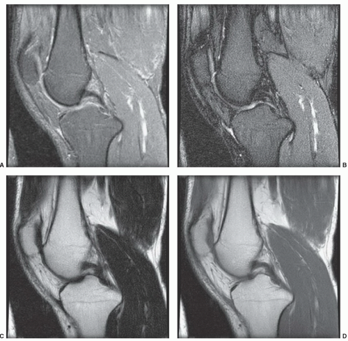 Figure 1.19 Image examples using the IR pulse sequence (magnitude reconstructions) with varying TI (TE = 14, 256 × 192, TR = 1500, 24 cm, 5 mm, 0.75 NEX, SAT on). A: TI = 100. B: TI = 170. C: TI = 400. D: TI = 800. |
FLOW AND MOTION COMPENSATION TECHNIQUES
Any movement of structures during MRI data acquisition can cause artifacts ranging from image “unsharpness” (as experienced in other modalities) to intense streaks that totally obscure the image. Such movements in patients can be caused by fluid flow or physiologic motion. Since the total sampling time in the phase encoding direction (TR x number of phase encoding steps) is substantially greater
than the sampling time in the frequency encoding direction (˜10 msec time frame), the amount of movement is much greater in the phase encoding direction. Image artifacts generally appear as linear bands in the phase encoding direction. Although the fundamental principles of physical movement during data acquisition are the same for both fluid flow and physiologic motion, the nature of each produces different artifacts and, therefore, different strategies are needed for motion artifact compensation.
than the sampling time in the frequency encoding direction (˜10 msec time frame), the amount of movement is much greater in the phase encoding direction. Image artifacts generally appear as linear bands in the phase encoding direction. Although the fundamental principles of physical movement during data acquisition are the same for both fluid flow and physiologic motion, the nature of each produces different artifacts and, therefore, different strategies are needed for motion artifact compensation.
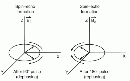 Figure 1.20 Spin-echo formation. A: Individual nuclei are precessing away from one another following 90° RF pulse. B: Individual nuclei are precessing toward one another following 180° (rephasing) RF pulse. |
Flow artifacts such as those shown in Figure 1.25 occur because the spins in the flowing blood accrue phase due to their movement in the presence of the gradient.13 Since the flow is not constant, the amount of accrued phase varies from view to view. The 2DFT image reconstruction translates this view-to-view phase variation to a distribution of intensities extending along the phase encoding direction (flow artifacts). Two approaches are often used to eliminate flow artifacts: gradient moment nulling (GMN) and spatial presaturation (SAT). Both techniques involve changes in the basic pulse sequence, yet provide different corrections. GMN14 essentially eliminates the phase accrual due to movement of spins, thereby decreasing the artifact and producing an image in which the vessel is of high intensity. SAT15 eliminates the high signal due to the inflow of fresh spins and produces an image with vessels of low intensity.
Related posts:

Stay updated, free articles. Join our Telegram channel

Full access? Get Clinical Tree


