ALBERT V. ARMSTRONG JR AND JACQUELINE M. BRILL
INTRODUCTION
Magnetic resonance imaging (MRI) has become the study of choice for many pathologic conditions of the musculoskeletal system.1 However, there are several situations when ultrasound becomes the imaging method of choice. Even though this is common knowledge in the imaging community, ultrasound is still underutilized by doctors of podiatric medicine.2 Box 26-1 lists the advantages of ultrasound over MRI. Aspiration of cysts, guided injections, and foreign body localization and removal can all be done in real time. Scanning can be done in virtually any plane; the examiner has complete control. With dynamic imaging, the transducer and the patient can be maneuvered to demonstrate pathology that may not be apparent on static images.3 Using the edge technique, the examiner can apply pressure with the transducer in an effort to reproduce the patient’s pain, thereby pinpointing the exact location of the pathology.4 Ultrasound examination of foot and ankle injuries has been advocated for the adult and pediatric populations.5
BOX 26-1 Advantages of Ultrasound over MRI: The ABC’s (ABCDE)
Aspiration, ultrasound-guided injections, foreign body localization/removal
B-mode real-time imaging
Cuts in multiple planes
Dynamic imaging
Edge technique
One of the disadvantages of using ultrasound is that it is operator dependant.6,7 Therefore, this chapter is designed as a scanning and positioning guide for foot and ankle anatomic structures. A detailed explanation of ultrasound physics is beyond the scope of this chapter. However, when evaluating the detailed anatomy and pathology of the foot and ankle, an understanding of the fundamental concepts of ultrasound physics and instrumentation is necessary. This will enhance one’s ability to successfully perform guided procedures, such as foreign body localization and removal and aspiration of joints and cysts. To perform such procedures successfully, one must be able to choose the appropriate instrument settings, identify appropriate anatomy, optimize one’s approach, and maximize the benefits of this technology.
INSTRUMENTATION
An ultrasound system consists of four main components: the electronic pulser, transducer, receiver, and display.8 The electronic pulser is the component that generates electricity that is sent to the transducer. The ultrasound transducer, also referred to as the probe, is the part of the ultrasound scanning device held by the user, and applied to the patient to generate an image. The term transducer is defined as a device that translates one form of energy to another. The portion of the transducer that converts the energy is called the piezoelectric crystal (piezo is pronounced pee-AY-zo). When an electrical charge is applied to the piezoelectric crystal it vibrates thus producing a mechanical wave of sound. Conversely, if a mechanical force is applied to the piezoelectric crystal, an electrical charge will be generated. These properties make the piezoelectric crystal ideal for the use of medical ultrasound because the same elements serve as both the transmitter and receiver of the ultrasound beam. Since most structures in the foot and ankle are superficial, one needs a linear array transducer, 10 MHz or above. Remember, increasing the frequency of sound increases resolution but decreases the depth of penetration. Therefore, a high-frequency transducer is necessary. The ultrasound system display will show the ultrasound image as well as other information such as the patient information, time and date of the exam, system settings, imaging depth, depth markers, transducer orientation marker, and type of transducer.
IMAGE ORIENTATION
To prevent disorientation, the physician must pay close attention to the transducer orientation. Though the width of the beam is equal to the width of the transducer, the thickness of the beam is only 1 mm wide. On the basis of standard radiology imaging conventions, the top of the screen is the transducer/patient contact point, and the bottom of the screen is distant or away from the skin surface, based on the depth setting. To properly keep the transducer oriented during scanning each transducer has an orientation mark on the outside plastic housing. The orientation mark on the transducer corresponds with the orientation marker on the display screen. For foot and ankle imaging, transverse and longitudinal images are most commonly obtained, though oblique planes can be obtained as well. For transverse images, the transducer orientation marker should always be positioned medially. On the display, therefore, the medial side of the patient will always correspond to the left side of the screen. For longitudinal images, the transducer orientation marker should always be placed proximally. On the display, therefore, the proximal structures on the patient will always correspond to the left side of the screen. By using this orientation, the structures visualized will always be on the same side of the screen, regardless if you are doing the right or left foot or ankle. In this chapter, when viewing an anatomic structure in cross section, we will use the terminology “short axis” whereas a longitudinal view will be termed “long axis” (Figure 26-1). Also remember, when scanning the plantar aspect of the foot you will be viewing the anatomy in the ultrasound images “upside down.” Therefore, the MRI comparison images in this chapter are also presented upside down.
Ultrasound images are created when the ultrasound beam is transmitted into the foot or ankle, and echoes are reflected back to the transducer from the various bones and soft tissue structures. When the beam reflects from a dense material such as bone, the image is bright and appears white on the screen (hyperechoic). When the ultrasound beam reflects from a more absorbing or softer structure, the image is darker or gray (hypoechoic) or black (anechoic). Think of a rubber ball bouncing off of different surfaces9:
• A white (hyperechoic) image results from a fast bounce off of a hard wall.
• A gray image results from a slow bounce off of a soft surface.
• A black image results when the ball fails to bounce back.
Bone surface appears bright white. Normal tendons appear white, but slightly darker than bone, and have a parallel grain fibrous pattern produced by fiber bundles. Tendons look like cables in long axis. In short axis, tendons display an acoustic property known as anisotropy.10 In addition, with tendonitis, the tendon will appear larger and darker than normal tendon (Figure 26-2). Muscle is darker than tendon, but also has a fibrous pattern due to bundles. Fascia is darker than bone, but brighter than muscle because it is denser. It may have the same brightness as muscle, but lacks the fibrous pattern because it has no fibrous bundles. Nerves, in short axis, will have a “honeycomb” appearance because it is made up of fascicles.
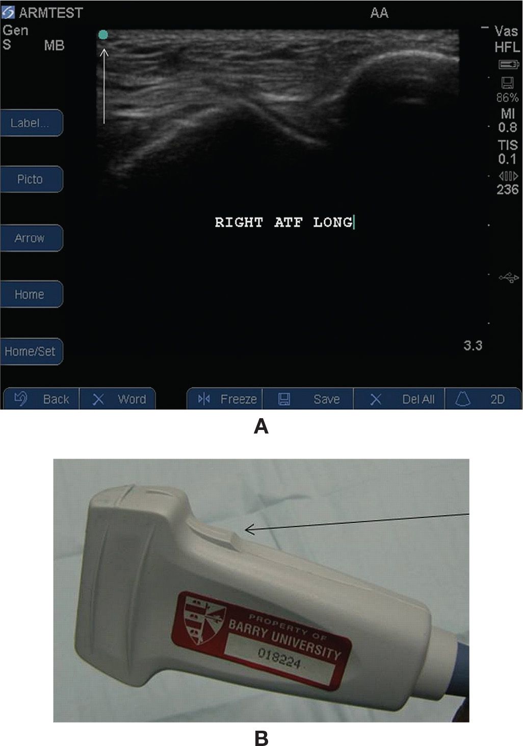
FIGURE 26-1. A: Image orientation marker (arrow). B: Transducer orientation marker (arrow).
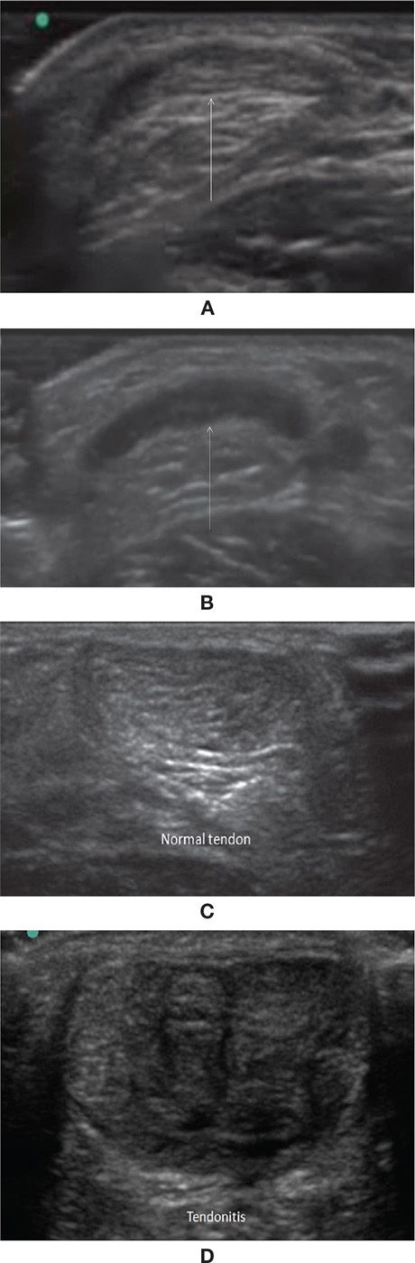
FIGURE 26-2. Anisotropy (arrows) demonstrated using the Achilles tendon in short axis. A: The transducer is 90° to the normal Achilles tendon. B: The transducer is at an angle other than 90° to the tendon. C: Normal proximal Achilles tendon. D: Same patient, with tendonitis in the distal Achilles tendon. Pain was reproduced using the “edge technique.”
ANATOMIC STRUCTURES
Anterior Talofibular Ligament—Long Axis (Figure 26-3)
Position of patient: Have the patient sit on the examining chair so that the foot and ankle are suspended off the edge.
Position of part: The patient should be resting Anterior Tibial Tendon comfortable so that the foot is slightly plantarflexed.
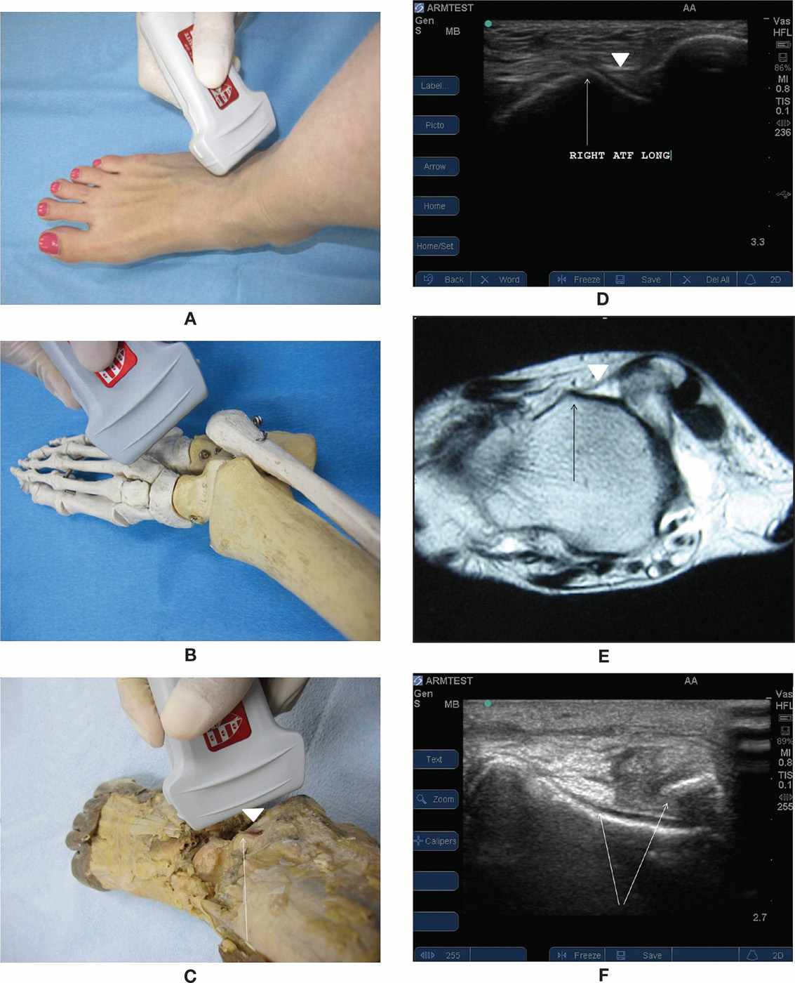
FIGURE 26-3. Anterior talofibular ligament. A: Position of patient. B: Skeletal model showing the position of the talus. C: Gross specimen. Arrow: the peak in the image is the talus, just inferior to the talar dome. Arrowhead: the anterior talofibular ligament. D: Ultrasound image (arrow and arrowhead as in C). E: MRI (arrow and arrowhead as in C). F: Ruptured anterior talofibular ligament (arrows).
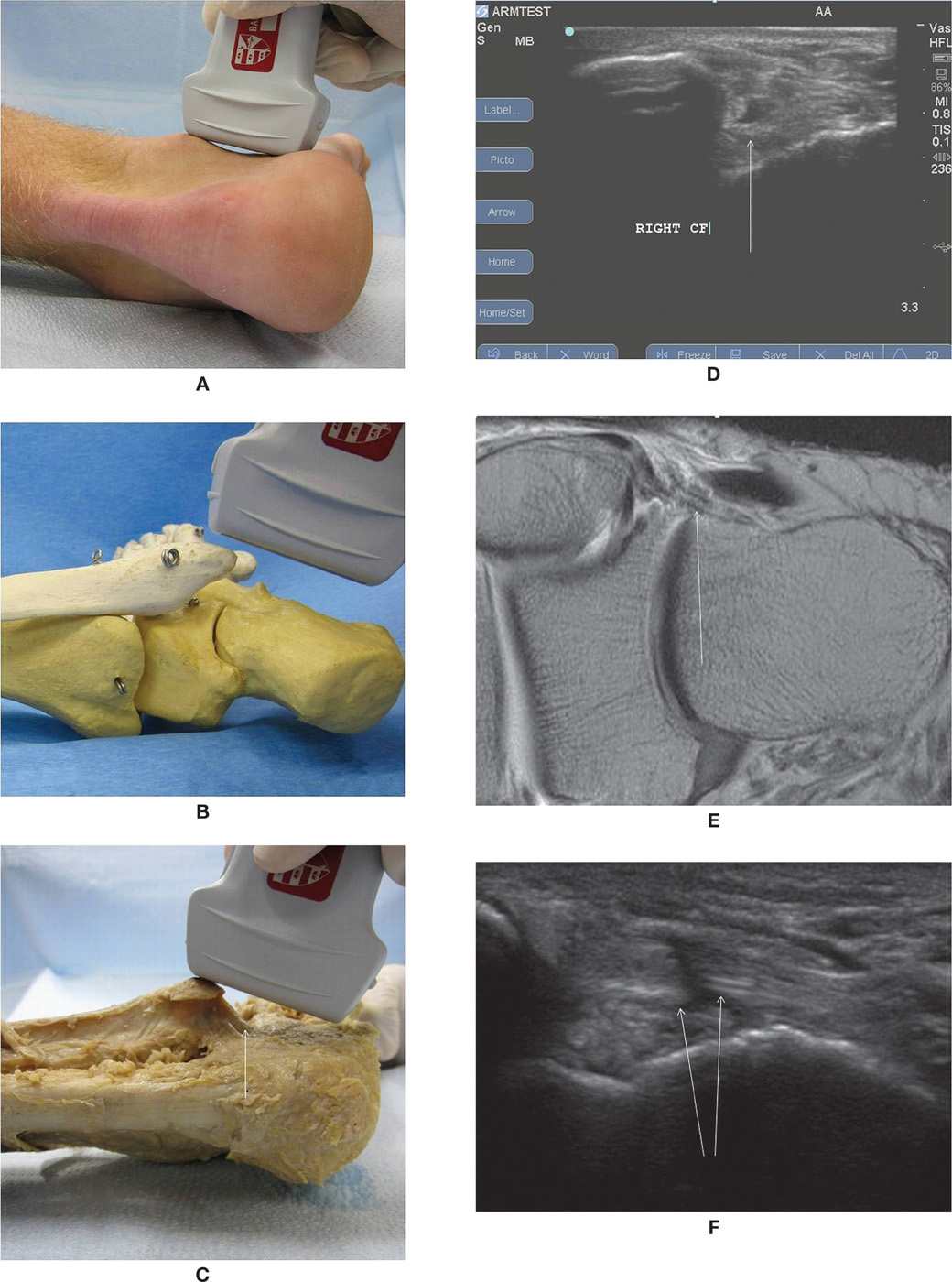
FIGURE 26-4. Calcaneofibular ligament (arrow). A: Position of patient. B: Skeleton model. C: Gross specimen. D: Ultrasound image. E: MRI. F: Ruptured calcaneofibular ligament.
Transducer position: Place the transducer on the lower ankle over the tibia and fibula, with the orientation mark pointing medially. Move the transducer distally until the fibula and inferior portion of the talus come into view.
Structures shown: Rounded edge of the anterior fibula. Inferior lateral edge of the talus (should appear as a “peak” in this view). Anterior talofibular ligament appears as an echogenic band between the fibula and talus.
Dynamic imaging: An anterior drawer manuver can be used under ultrasound to further evaluate ligamentous integrity.
Calcaneofibular Ligament—Long Axis (Figure 26-4)
Position of patient: The patient should be lying on the opposite hip of the ankle to be scanned.
Position of part: Lateral side of the ankle to be scanned up.
Transducer position: Place the transducer over the lateral malleolus and the calcaneus, with the orientation mark oriented proximally, and pointed at approximately at 2 o’clock.
Structures shown: Rounded inferior edge of the fibula. Calcaneofibular ligament in long axis. Lateral wall of the calcaneus
Dynamic imaging: Inverting the foot under ultrasound can be done to further evaluate ligamentous integrity (Figure 26-4F).
Peroneal Tendons—Short Axis (Figure 26-5)
Position of patient: The patient should be lying on the opposite hip of the ankle to be scanned.
Position of part: Lateral side of the ankle to be scanned up.
Transducer position: Place the transducer on the posterior lower leg over the fibula. The orientation mark should be directed medially.
Structures shown: Rounded posterior edge of the fibula. Peroneus longus and brevis tendons in short axis.
Dynamic imaging: Dorsiflexion and eversion of the ankle can help demonstrate dislocatable peroneal tendons.11
Peroneal Tendons—Long Axis (Figure 26-6)
Position of patient: The patient should be lying on the opposite hip of the ankle to be scanned.
Position of part: Lateral side of the ankle to be scanned up.
Transducer position: Place the transducer on the posterior lower leg, just posterior to the fibula. The orientation mark should be directed proximally.
Structure shown: Peroneus longus and brevis tendons in long axis.
Anterior Tibial Tendon—Short Axis (Figure 26-7)
Position of patient: Supine or sitting up in the examining chair.
Position of part: Patient can rest comfortably with the foot slightly plantarflexed.
Transducer position: Place the transducer on the anterior ankle. The orientation mark should be directed medially.
Structure shown: Tibialis anterior tendon in short axis.
Anterior Tibial Tendon—Long Axis (Figure 26-8)
Position of patient: Supine or sitting up in the examining chair.
Position of part: Patient can rest comfortably with the foot slightly plantarflexed.
Transducer position: Place the transducer on the anterior ankle. The orientation mark should be directed proximally.
Structure shown: Tibialis anterior tendon in long axis.
Posterior Tibial Tendon/Flexor Digitorum Longus Tendon/Tibial Neurovascular Bundle/Flexor Hallucis Longus Tendon—Short Axis (Figure 26-9)
Position of patient: Have patient turn onto the hip of the ankle to be scanned.
Position of part: Medial side of the ankle up.
Transducer position: Place the transducer over medial ankle, with the orientation mark directed medially. Make sure the orientation mark edge of the transducer is over the posterior tibia, with the remaining portion of the probe posterior to the tibia.
Structures shown: Rounded medial edge of the tibia. Laciniate ligament. Posterior tibial tendon and flexor digitorum longus tendon adjacent to each other in short axis. Posterior tibial neurovascular bundle. Flexor hallucis longus tendon in short axis.
Dynamic imaging: Dorsiflexion and inversion of the ankle can help demonstrate a dislocatable posterior tibial tendon.12
Posterior Tibial Tendon/Flexor Digitorum Longus Tendon—Long Axis (Figure 26-10)
Related posts:

Stay updated, free articles. Join our Telegram channel

Full access? Get Clinical Tree


