Shape Modeling of Musculoskeletal Structures and Its Applications

Fig. 1

Transformation of a human into a rhinoceros head is made possible through the representation of shapes in a common shape space

Is is obvious that the details of the correspondence identification has a great impact on subsequent analysis, see Fig. 2. Nevertheless, a proper definition for “good” correspondences is difficult to establish in general, and in most cases must be provided in the context of the application. One generic approach to establish correspondence, however, optimizes the resulting statistical shape model built from the correspondences, i.e. its compactness or generalization ability, see Sect. 2.4. Refer to Davies et al. [3] for more details.

Fig. 2

When the tip of the nose on the left head is matched with a point on the cheek on the right head, shape interpolation may yield a head with two noses

2.3 Statistical Analysis

As soon as we are able to perform “shape arithmetic” in a shape space, we can perform any kind of statistical analysis, e.g. like principal component analysis (PCA). This kind of analysis takes as input a set of training shapes S ₁, …, S _nand extracts the so-called modes of variations V ₁, …, V _n−1 sorted by their variance in the training set. Together with the mean shape $\overline{S}$ the modes of variations form a statistical shape model (SSM):

$S(b_{1} , \ldots ,b_{n - 1} ) = \overline{S} + \sum\limits_{k = 1}^{n - 1} b_{k} \cdot V_{k}$

(1)

The SSM is a family of shapes determined by the parameters b ₁, …, b _n−1, each of which weights one of the modes of variations V _k. For instance, if we set b ₂ = ··· = b _n−1 = 0 and vary only b ₁ we will see the effect of the first mode of variation on the deformations of the shapes within the range of the training population. The PCA may be exchanged with other methods, which will alter the interpretation of both the V _kand their weights b _k. See Sect. 3.3.2 for such an alternative approach.

In the PCA case, the idea is that the variance within the training population is contained in only few modes, hence the whole family of shapes can be described with only a few “essential degrees of freedom”, see Fig. 3. Note that the shape variations V _iare generally global deformations of the shape, i.e. they vary every point on the shape. Thus, a SSM can be a highly compact representation of a family of complex geometric shapes. Furthermore, it is straightforward to synthesize new shapes by choosing new weights. These may lie within the range of the training shapes or even extrapolate beyond that range.

Fig. 3

Left Overlay of several training shapes. Middle First three modes of variation from top to bottom. Local deformation strength is color-coded. Right 90 % variation lie within 15 shape modes

2.4 Evaluation

With the SSM we can represent any shape as a linear combination of the input shapes or some kind of transformation of those input shapes, e.g. via PCA. However, up to what accuracy can we represent/reconstruct an unknown shape S ^* by an SSM S(b)? The idea is to compute the best approximation of the SSM to the unknown shape:

$b^{*} = \mathop {\text{argmin}}\limits_{b} d(S^{*} ,S(b))$

(2)

where d(·, ·) is a measure for the distance between two shapes. Then S(b ^*) is the best approximation of S ^* within the SSM.

If d(S ^*, S(b ^*)) = 0 then the unknown shape is already “contained” in the SSM, otherwise the SSM is not capable of explaining S ^*. The smaller d(S ^*, S(b ^*)) for any S ^*, the higher the so-called generalizability of the SSM. A better generalizability can be achieved by including more training samples into the model generation process. A good SSM has a high generalizability or reconstruction capability. On the other hand, if S(b) for an arbitrary b is similar to any of the training data sets S ₁, …, S _n, the SSM is said to be of high specificity. In other words, synthesized shapes do indeed resemble real members of the training population. Generalizability and specificity need to be verified experimentally.

3 Applications

3.1 Anatomy Reconstruction

One of the basic challenges in processing medical image data is the automation of segmentation or anatomy reconstruction. Due to noise, artifacts, low contrast, partial field-of-view and other measurement-related issues, the automatic delineation and discrimination of specific structures from other structures or the background—seemingly an easy task for the human brain—is still challenging for the computer.

However, over the last two decades, model-based approaches have shown to be effective to tackle this challenge, at least for well-defined application-specific settings. The basis idea is the use a deformable shape template (such as a SSM) and match it to medical image data like CT or MRI. In this case, the shape S ^* from Eq. (2) is not known explicitly. Therefore, such an approach—in addition to the SSM—requires a intensity model, that quantifies how well an instance of the SSM fits to the image data, see Fig. 4. From such a model, S ^* can be estimated. Many such intensity models have been proposed in the literature. One generic approach is to “learn” such a model from training images similar to the way SSMs are generated [2]. Shape models are also combined with intensity models in SSIMs or shape and appearance Models. An overview can be found in [10].

Fig. 4

A SSM is matched to CT data. At each point of the surface an intensity models predicts the desired deformation

The strength of this approach is its robustness stemming from the SSM. Only SSM instances can be reconstructed, thus this method can successfully cope with noisy, partial, low-dimensional or sparse image data.

On the other hand, since the SSM is generally limited in its generalization capability, some additional degrees of freedom are often required in order to get a more accurate reconstruction. Here, finding a trade-off between robustness and accuracy remains an issue. One successful approach for achieving such a trade-off are so called omni-directional displacements [13], see Fig. 5.

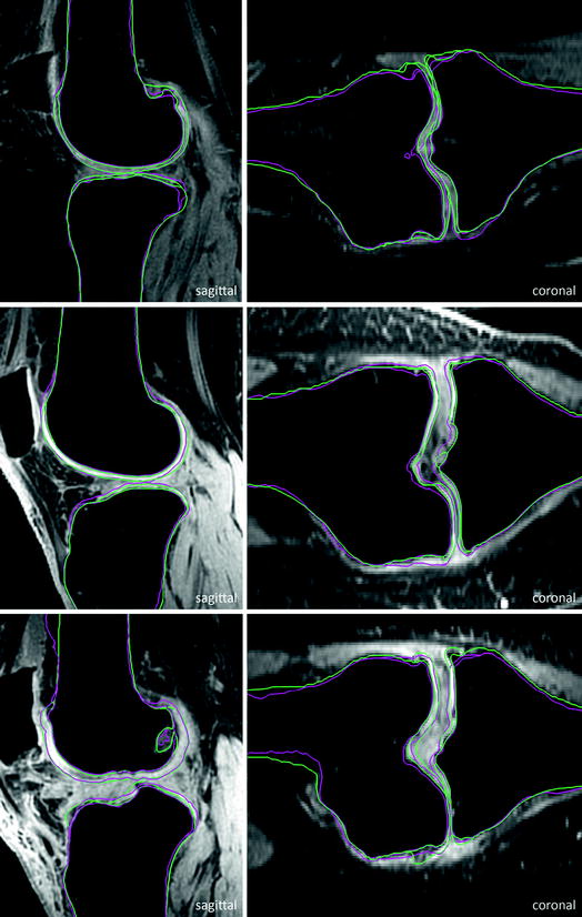
Fig. 5

Instead of just normal displacements as shown in Fig. 4, omnidirectional displacements allow for much more flexibility of local deformations, e.g. in regions of high curvature consistent local translations can be modeled

Fig. 6

Selected test cases sorted by quality in terms of achieved score. Top to bottom bad case, medium case, and good case. Pink Automatic segmentation. Green Ground truth (Color figure online)

3.1.1 Example: Knee-Joint Reconstruction from MRI

Osteoarthritis (OA) is a disabling disease affecting more than one third of the population over the age of 60. Monitoring the progression of OA or the response to structure modifying drugs requires exact quantification of the knee cartilage by measuring e.g. the bone interface, the cartilage thickness or the cartilage volume. Manual delineation for detailed assessment of knee bones and cartilage morphology, as it is often performed in clinical routine, is generally irreproducible and labor intensive with reconstruction times up to several hours.

Seim et al. [20] present a method for fully automatic segmentation of the bones and cartilages of the human knee from MRI data. Based on statistical shape models and graph-based optimization, first the femoral and tibial bone surfaces are reconstructed. Starting from the bone surfaces the cartilages are segmented simultaneously with a multi-object technique using prior knowledge on the variation of cartilage thickness.

For evaluation, 40 additional clinical MRI datasets acquired before knee replacement are available. A detailed evaluation is presented in Fig. 7. For tibial and femoral bones the average (AvgD) and the roots mean square (RMS) surface distances were computed. Cartilage segmentation is quantified by volumetric overlap (VOE) and volumetric difference (VD) measures. For all four structures a score was computed indicating the agreement with human inter-observer variability. Reaching the inter-observer variability results in 75 points, while obtaining an exact match to one distinguished manual segmentation results in 100 points. An error twice as high as the human rater’s gets 50 points, 3× as high gets 25 points and if 4× as high or more receives 0 points (no negative points). All points are averaged for each image, which results in a total score per image. Details on the evaluation procedure are published in an overview article of the Grand Challenge workshop (www.grand-challenge.org). The average performance of our auto-segmentation system for knee bones and associated cartilage was 64.4 ± 7.5 points. Exemplary results are shown in Fig. 6.

Fig. 7

Evaluation of automatic segmentations against ground truth for 40 training datasets

The bone segmentation achieves scores that indicate an error larger than that obtained by human experts. This may be due to relatively large mismatches of the SSM at the proximal and distal end of the MRI data due to missing or weak image features related to intensity inhomogeneities stemming from the MRI sequence (see Fig. 8). A strong artifact of unknown source (see Fig. 8) lead to the worst segmentation result for the tibia. The scores for cartilage segmentation are based on different error measures (volumetric) and are generally better, presumably due to a higher inter-observer variability.

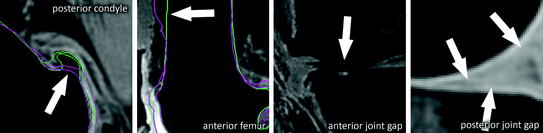
Fig. 8

Challenging regions: large osteophytes with high curvature, low contrast at anterior bone-shaft to soft-tissue interface, strong cartilage wear, low contrast at cartilage to soft-tissue interface, under-segmented bone at cartilage interface

3.1.2 Example: 3D Reconstruction from X-ray

The orientation of the natural acetabulum is useful for total hip arthroplasty (THA) planning and for researching acetabular problems. Currently the same acetabular component orientation goal is generally applied to all THA patients. Creating a patient-specific plan could improve the clinical outcome. The gold standard for surgical planning is from threedimensional (3D) computed tomography (CT) imaging. However, this adds time and cost, and exposes the patient to a substantial radiation dose. If the acetabular orientation could be reliably derived from the standard anteroposterior (AP) radiograph, preoperative planning would be more widespread, and research analyses could be applied to retrospective data, after a postoperative issue is discovered. The reduced dimensionality in 2D X-ray images and its perspective distortion, however, lead to ambiguities that render an accurate assessment of the orientation parameters a difficult task. One goal is to enable robust measurement of the acetabular inclination and version on 2D X-rays using computer-aided techniques.

Based on the idea of Lamecker et al. [17], Ehlke et al. [4] propose a reconstruction method to determine the natural acetabular orientation from a single, preoperative X-ray. The basic idea is to take virtual X-rays of a (extended) SSM and compare them to a clinical X-ray in an optimization framework. The best matching model instance gives an estimated shape and pose (and bone density distribution) of the subject (Fig. 9). The acetabular orientation (Fig. 10) can then be assessed directly from the reconstructed, patient specific anatomy model [5, 6]. The approach utilizes novel articulated statistical shape and intensity models (ASSIMs) that express the variance in anatomical shape and bone density of the pelvis/proximal femur between individual patients and model the articulation of the hip joints.

Fig. 9

The 3D shape reconstruction process from X-ray images optimizes the similarity between virtual X-ray images generate from the SSIM with the clinical X-ray images