Fig. 1
Characteristics of rigid registration spatial errors: a corresponding points (1a–2a, 1b–2b) before registration; after registration b error only in translation, c error only in rotation. In both cases it is clear that registration reduced the spatial error between the points. It is also clear that the effect of the translational error on the spatial errors is uniform throughout space, while the effect of the rotational error depends on the distance from the origin. In theory, one can eliminate the effect of rotational errors for a single point by placing the origin of the reference frame at this point of interest
While developers of registration frameworks strive to construct the ideal framework, this is not an easy task. More importantly, it is context dependent. For example, introducing an US machine for the sole purpose of registration makes the framework non-ideal. On the other hand, if the US machine is already available, for instance to determine breaches in pedicle screw hole placement [52], utilizing it for registration purposes does not preclude the framework from being considered ideal.
Given that constructing the ideal framework is hard, it is only natural that developers of guidance systems have devised schemes that bypass this task. We thus start our overview of registration in orthopedics with approaches that perform registration implicitly.
2 Implicit Registration
We identify two distinct approaches to performing implicit registration. The first combines preoperative calibration with intraoperative volumetric image acquisition using cone-beam CT (CBCT). The second uses patient specific templates that are physically mounted onto the patient in an accurate manner. These devices physically constrain the clinician to planned trajectories for drilling or cutting.
2.1 Intraoperative CBCT
This approach relies on the use of a tracked volumetric imaging system to implicitly register the acquired volume to a Dynamic Reference Frame (DRF) rigidly attached to the patient. During construction of the imaging device, it is calibrated such that the location and orientation of the reconstructed volume is known with respect to a DRF that is built into the system. Intraoperatively, a volumetric image is acquired while the patient’s DRF and imaging device’s DRF are both tracked by a spatial localization system. This allows the navigation system to correctly position and orient the volume in physical space. It should be noted that some manufacturers refer to this registration bypass as automated registration, although strictly speaking the system is not performing intraoperative registration. Figure 2 shows an example of the physical setup and coordinate systems involved in the use of such a system.
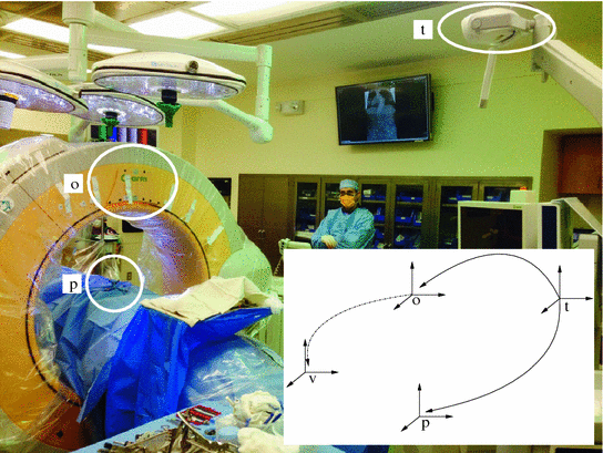
Fig. 2
The O-arm system from Medtronic (Minnisota, MN, USA) facilitates implicit registration via factory calibration. Picture shows the clinical setup (Courtesy of Dr. Matthew Oetgen, Children’s National Health System, USA). Inset shows corresponding coordinate systems and transformations. Transformations from tracking coordinate system, t, to patient DRF, p, and O-arm DRF, o, vary per procedure and are obtained from the tracking device. The transformation between the O-arm DRF, o, and the volume coordinate system acquired by the O-arm, v, is fixed and obtained via factory calibration. Once the volume is acquired intraoperatively it is implicitly registered to the patient as the transformation from the patient to the volume is readily constructed by applying the three known transformations
These systems have been used to guide various procedures for a number of anatomical structures including the hip [11, 118], the foot [101], the tibia [134], the spine [23, 38, 53, 83, 107], and the hand [115].
When compared to our ideal registration framework these systems satisfy almost all requirements. They are accurate and precise with submillimetric performance. They are robust, although the use of optical tracking devices means that they are dependent on an unobstructed line of sight both to the patient’s and device’s DRFs. They provide the desired transformation in less than 1 s, as almost no computation is performed intraoperatively after image acquisition. These systems are not obtrusive as they are used to acquire both intraoperative X-ray fluoroscopy and volumetric imaging. The one criterion where they can be judged as less than ideal is that these systems expose the patient to ionizing radiation.
While these systems offer many advantages when evaluated with regard to components of the registration framework, they do have other limitations. The quality of the volumetric images acquired by these devices is lower than that of diagnostic CT images and this can potentially have an effect on the quality of the visual guidance they provide. Obviously, one can register preoperative diagnostic images (CT, PET, MR) to the intraoperative CBCT, but this changes the registration framework and it is unclear whether such a system retains the advantages associated with the existing one. Another, non technical, disadvantage is the cost associated with these imaging systems. They do increase the overall cost of the navigation system. One potential approach to addressing the cost of high end CBCT systems is to retrofit non-motorized C-arm systems to perform CBCT reconstructions. This requires that the position and orientation of the C-arm be known for each of the acquired X-rays during a manual rotation. Two potential solutions to this task have been described in the literature. The C-Insight system from Mazor Robotics (Caesarea, Israel) [134] uses an intrinsic tracking approach. It both calibrates the X-ray system and estimates the C-arm pose using spherical markers visible in the X-ray images. An extrinsic approach to tracking is describe in [2]. This system utilizes inertial measurement units attached to a standard C-arm to obtain the pose associated with each image. As both approaches retrofit standard C-arms the quality of the reconstructed volumes is expected to be lower than those obtained with motorized CBCT machines, as these also utilize flat panel sensors which yield higher quality input for CBCT reconstruction.
2.2 Patient Specific Templates
This approach relies on the use of physical templates to guide cutting or drilling. The templates are designed based on anatomical structures and plans formulated using preoperative volumetric images, primarily diagnostic CT. This is in many ways similar to stereotactic brain surgery, using patient mounted frames. To physically guide the surgeon the template incorporates two components, the bone contact surface which is obtained via segmentation from the preoperative image and guidance channels which correspond to the physical constraints specified by the plan. Templates can be created either via milling, subtractive fabrication, or via 3D printing, additive fabrication. The later approach has become more common as the costs of 3D printers have come down. Figure 3 illustrates this concept in the context of pedicle screw insertion.
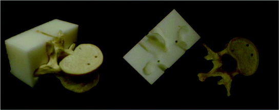
Fig. 3
Patient specific 3D printed template for pedicle screw insertion. Template incorporates drill trajectories planned on preoperative CT (Courtesy Dr. Terry S. Yoo, National Institutes of Health, USA)
Patient specific templates have been used to guide various procedures for a number of anatomical structures including the spine [15, 68, 69, 98], the hand [60, 70, 85], the hip [41, 98, 119, 148], and the knee [43, 98].
When compared to the ideal registration framework, this approach provides sufficient accuracy, precision and robustness. Registration is obtained implicitly in an intuitive manner, as the template is manually fit onto the bone surface. This approach is not obtrusive as it does not require additional equipment other than the template. In theory there are no clinical side effects associated with the use of a template. Unfortunately, achieving accuracy, precision and robustness requires that the template fit onto the bone in a unique configuration. This potentially requires a larger contact surface, resulting in larger incisions than those used by standard minimally invasive approaches [119]. While a smaller contact surface is desirable it should be noted that this will potentially increase the chance that the operator “fits the square peg into a round hole” (e.g. wrong-level fitting for pedicle screw insertion).
3 3D/3D Registration
In orthopaedics, 3D/3D registration is utilized for alignment of preoperative data to the physical world, spatial alignment of data as part of procedure planning, and for construction of statistical shape and appearance models with the intent of replacing the use of preoperative CT for navigation with a patient specific model derived from the statistical one.
Alignment of preoperative data to the physical world is the most common usage of registration in orthopaedics. It has been described as a component of robotic procedures applied to the knee [7, 67, 78, 79, 96, 103], and hip [73, 81, 109]. In the context of image-guided navigation, it has been described as a component of procedures in the hip [8–10, 54, 61, 94, 110, 118, 119], the femur [8, 16, 94, 99, 154], the knee [54, 99, 116], and the spine [31, 46, 61, 100, 120, 143].
In the context of planning, 3D/3D registration has been used for population studies targeting implant design [58], for the selection and alignment of a patient specific optimal femoral implant in total hip arthroplasty [90], and for planning the alignment of multiple fracture fragments using registration to the contralateral anatomy, thus enabling automated formulation of plans in distal radius osteotomy [27, 28, 102, 111], humerus fracture fixation [14, 35], femur fracture fixation [86] and potentially for scaphoid fracture fixation [63].
In the context of statistical model creation, the first journal publications to describe the use of statistical shape models in orthopedics were [34, 117]. The motivation for this work was to create a patient specific model for guiding ACL reconstruction and total knee arthroplasty without the need of a preoperative 3D scan. A statistical point distribution model of the distal part of the femur was created by digitizing the surfaces of multiple dry bone specimens and creating the required anatomical point correspondence via non-rigid 3D/3D registration. Many others follow a similar approach but with one primary difference, the models used to describe the population are obtained from previously acquired 3D scans, CT or MR, of other patients. This allows modeling of both shape and intensity. For a detailed overview of the different aspects of constructing statistical shape models we refer the interested reader to [44].
In orthopedics, statistical shape models that use registration for establishing anatomical point correspondences have primarily used the free-form deformation method proposed in [104] and the diffeomorphic-demons method proposed in [131]. These registration methods were utilized for creating models of the femur, pelvis and tibia [9, 16, 58, 108, 137, 147]. This approach was also recently applied in 2D, using 2D/2D registration to establish point correspondences for a proximal femur model [140]. Figure 4 shows the resulting 2D statistical point distribution model.
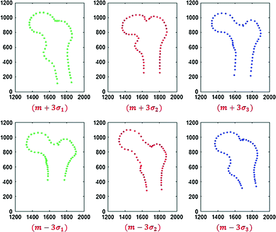
Fig. 4
2D proximal femur statistical point distribution model, three standard deviations from the mean shape, along the first three modes of variation (Courtesy Dr. Guoyan Zheng, University of Bern, Switzerland)
At this point we would like to highlight two aspects associated with the use of statistical point distribution models which one should always think about: does the input to the statistical model truly reflect the population variability (e.g. using femur data obtained only from females will most likely not reflect the shape and size of male femurs); and if point correspondences were established using registration, how accurate and robust was the registration method.
Having motivated the utility of 3D/3D registration in orthopedics, we now turn our attention to several common algorithms, pointing out their advantages and limitations.
3.1 Point Set to Point Set Registration
In this section we discuss three common algorithm families used to align point sets in orthopedics, paired-point algorithms, surface based algorithms and statistical surface models.
Paired-point algorithms use points with known correspondences to compute the rigid transformation between the two coordinate systems. In this setting points are localized, most often, manually both in image space via mouse clicks, and in physical space via digitizing using a tracked calibrated pointing device such as described in [122]. Both calibration and tracking of pointer devices can be done with sub-millimetric accuracy.
In general, we are given three or more corresponding points in two Cartesian coordinate systems:
 where
where  are the true point coordinates related via a rigid transformation
  ,
,  are the observed coordinates, and
  are the errors in localizing the points.
are the true point coordinates related via a rigid transformation , are the observed coordinates, and are the errors in localizing the points.The most common solution to this problem is based on a least squares formulation:
The solution to this formulation is optimal if we assume that there are no outliers and that the Fiducial Localization Errors (FLE)1 follow an isotropic and homogenous Gaussian distribution. That is, the error distribution is the same in all directions and is the same for all fiducials. Figure 5 visually illustrates the possible FLE categories.
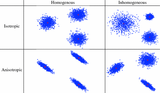
Fig. 5
Categories of fiducial localization error according to their variance. Plus (red) indicates fiducial location and star/circle/triangle marks (blue) denote localization variability (Color figure online)
While the formulation is unique, several analytic solutions have been described in the literature, with the main difference between them being the mathematical representation of rotation. These include use of a rotation matrix [3, 128], a unit quaternion [32, 47], and a dual quaternion [132]. All of these algorithms guarantee a correct registration if the assumptions hold. Luckily, empirical evaluation has shown that all choices yield comparable results [30].
In practice, FLE is often anisotropic, such as when using optical tracking systems, where the error along the camera’s viewing direction is much larger than the errors perpendicular to it [138]. In this case, the formulation described above does not lead to an optimal solution. Iterative solutions addressing anisotropic-homogenous noise and anisotropic-inhomogeneous noise models were described in [77, 84] respectively. These methods did not replace the least squares solutions even though they explicitly address the true error distributions. This is possible due to two attributes of the original algorithms, they are analytic, that is they do not require an initial solution as iterative algorithms do, and they are extremely easy to implement. Case in point, Table 1 is a fully functioning implementation of the method described in [128] using MATLAB (The Mathworks Inc., Natick, MA, USA).
Table 1
Source code shows complete implementation of analytic paired point rigid registration in MATLAB
function T = absoluteOrientation(pL, pR) |
n = size(pL,2); meanL = mean(pL,2); meanR = mean(pR,2); [U,S,V] = svd((pL – meanL(:,ones(1,n))) * (pR – meanR(:,ones(1,n)))′); R = V*diag([1,1,det(U*V)])*U′; t = meanR – R*meanL; T = [R, t; [0, 0, 0, 1]]; |
One of the issues with paired-point registration methods is that the pairing is explicit, that is the clinician has to indicate which points correspond. This is often performed as part of a manual point localization process which is known to be inaccurate both in the physical and the image spaces [46, 112]. The combination of fixed pairing and localization errors reduces the accuracy of registration, as we are not truly using the same point in both coordinate systems. If on the other hand we allow for some flexibility in matching points then we may improve the registration accuracy. This leads directly to the idea of surface based registration.
Preoperative surfaces are readily obtained from diagnostic CT. Intraoperative surface acquisition is often done using a tracked pointer probe [4]. To ensure registration success one must acquire a sufficiently large region so that the intraoperative surface cannot be ambiguously matched to the preoperatively extracted one. This is a potential issue if it requires increased exposure of the anatomy only for the sake of registration. A possible non-invasive solution is to use calibrated and tracked ultrasound (US) for surface acquisition. US calibration is still an active area of research with multiple approaches described in the literature [76], most yielding errors on the millimeter scale. More recently published results report sub-millimetric accuracy [80]. Once the tracked calibrated US images are acquired, the bone surface is segmented in the images and its spatial location is computed using the tracking and calibration data. Automated segmentation of the bone surface is not a trivial task. In the works described in [8, 9] the femur and pelvis were manually segmented in the US images prior to registration, this is not practical for clinical use. Automated bone surface segmentation algorithms in US images have been described in [54, 57, 100, 110, 120] for B-mode US and in [79] for A-mode. These algorithms were evaluated as part of registration frameworks which have clinically acceptable errors (on the order of 2 mm).
Surface based registration algorithms use points without a known correspondences to compute the rigid transformation between the two coordinate systems. A natural approach for scientists tackling such problems is to decompose them into sub problems with the intent of using existing solutions for each of the sub problems. This general way of thinking is formally known as “computational thinking” and is a common approach in computer science [139].
Given that we have an analytic algorithm for computing the transformation when we have a known point pairing it was only natural for computer scientists to propose a two step approach towards solving this registration task. First match points based on proximity and then estimate the transformation using the existing paired-point algorithm. This process is repeated iteratively with the incremental transformations combined until the two surfaces are in correspondence. This algorithmic approach is now known as the Iterative Closest Point (ICP) algorithm. This algorithm was independently introduced by several groups [13, 20, 149].
While the simplicity of the ICP algorithm makes it attractive, from an implementation standpoint, it has several known deficiencies. The final solution is highly dependent on the initial transformation estimate, and speed is dependent on the computational cost of point pairing. In addition, the use of the analytic least squares algorithm to compute the incremental transformations assumes that there are no outliers and that the error in point localization is isotropic and homogenous. Many methods for improving these deficiencies have been described in the literature, with a comprehensive summary given in [105]. One aspect of the ICP algorithm that was not addressed till recently was that the localization errors are often anisotropic and inhomogeneous. A variant of ICP addressing this issue was recently described in [72].
From a practical standpoint, a combination of paired-point and an ICP variant is often used. The analytic solution most often provides a reasonable initialization for the ICP algorithm which then provides improved accuracy. This was shown empirically in [46]. Unfortunately, this combination still does not guarantee convergence to the correct solution. This is primarily an issue when the intraoperatively digitized surface is small when compared to the preoperative surface. In this situation the surface registration may be trapped by multiple local minima. This is most likely the reason for the poor registration results reported in [4] for registering the femur head in the context of hip arthroscopy.
Statistical surface model based registration [34, 117] are similar to surface based registration as described above, but with one critical difference, they do not use patient specific preoperative data. Instead of a patient specific surface obtained from CT, a surface model is created and aligned to the intraoperative point cloud. The statistical model encodes the variability of multiple example bone surfaces and uses the dominant modes of variation to fit a patient specific model to the intraoperative point cloud. An advantage of using such an approach is that models created from the atlas are limited to the variations observed in the data used to construct it. Thus, these models are plausible. Unfortunately, they often will not provide a good fit to previously unseen pathology. This can be mitigated by allowing the model to locally deform in a smooth manner to better fit the intraoperative point cloud [117].
3.2 Intensity Based Registration
Intensity based registration aligns two images by formulating the task as an optimization problem. The optimized function is dependent on the image intensity values and the transformation parameters. As the intensity values for the images are given at a discrete set of grid locations and the transformation is over a continuous domain, registration algorithms must interpolate intensity values at non grid locations. This means that all intensity based registration algorithms include at least three components: (1) The optimized similarity function which indicates how similar are the two images, subject to the estimated transformation between them; (2) An optimization algorithm; and (3) an interpolation method.
A large number of similarity measures have been described in the literature and are in use. Selecting a similarity measure is task dependent with no “best” choice applicable to all registration tasks. The selection of a similarity measure first and foremost depends on the relationship between the intensity values of the modalities being registered. When registering data from the same modality one may use the sum of squared differences or the sum of absolute differences. For modalities with a linear relationship between them one may use the normalized cross correlation. For modalities with a general functional relationship one can use the correlation ratio. Finally, for more general relationships, such as the probabilistic relationship between CT and PET one may use mutual information or normalized mutual information. These last similarity measures assume the least about the two modalities and are thus widely applicable. This does not mean that they are optimal, as we are ignoring other relevant evaluation criteria: computational complexity, robustness, accuracy, and convergence range. Incorporating domain knowledge when selecting a similarity measure usually improves all aspects of registration performance. More often than not, selecting a similarity measure should be done in an empirical manner, evaluating the selection on all relevant criteria. Case in point, the study of similarity measures described in [92] for 2D/3D registration of X-ray/CT.
Optimization is a mature scientific field with a large number of algorithms available for solving both constrained and unconstrained optimization tasks [33]. The selection of a specific optimization method is tightly coupled to the characteristics of the optimized function. For example, if the similarity measure is discontinuous using gradient based optimization methods is not recommended.
Finally, selecting an interpolation method is dependent on the density of the original data. If the images have a high spatial sampling, we can use simpler interpolation methods as the distance between grid points is smaller. With current imaging protocols linear interpolation often provides sufficiently accurate estimates in a computationally efficient manner. Obviously, other higher order interpolation methods can provide more accurate estimates with a higher computational cost [62].
In orthopedics 3D/3D intensity based non-rigid registration has been used for creating point matches for point distribution based statistical atlases. These models encode the variability of bone shape via statistics on point locations across the population. This in turn assumes that the corresponding points can be identified in all datasets. For sparse anatomically prominent landmarks this can potentially be done manually. For the dense correspondence required to model anatomical variability this is not an option. If on the other hand we non-rigidly align the volumetric data we can propagate a template mesh created from one of the volumes to the others, implicitly establishing the dense correspondence. In [9] this is performed using the free-form deformation registration approach with normalized mutual information as the similarity measure. In [16, 108] registration is performed with a diffeomorphic-demons method with the former using a regularization model which is tailored for improving registration of the femur. It should be noted that the demons set of algorithms assume the intensity values for corresponding points are the same for the two modalities. Finally, in [58] registration is performed using the free-form deformation algorithm and the sum of squared differences similarity measure.
Another setting in which 3D/3D intensity based rigid registration has been utilized in orthopedics is for alignment of preoperative data to the physical world, using intraoperative tracked and calibrated US to align a preoperative CT. In [94] both the US and CT images are converted to probability images based on the likelihood of a voxel being on the bone surface, with the similarity between the probability images evaluated using the normalized cross correlation metric. In [36, 61] simulated US images are created from the CT based on the current estimate of the US probe in the physical world. In both cases simulation of US from CT follows the model described in [135]. Registration is then performed using the Covariance Matrix Adaptation Evolution Strategy, optimizing the correlation ration in the former work and a similarity measure closely related to normalized cross correlation in the later work. In [141, 142] coarse localization of the bone surface is automatically performed both in the CT and US with the intensity values in the respective regions used for registration using the normalized cross correlation similarity measure. To date, US based registration has not become part of clinical practice. This is primarily due to the fact that US machines are not readily available in the operating room as part of current orthopedic procedures. Requiring the availability of additional hardware only for the sake of registration appears to limit adoption of this form of registration.
Related posts:
 of Implant Osseointegration by Means of a Reconstruction Algorithm on Micro-computed Tomography Images
Fusion for Computer-Assisted Bone Tumor Surgery
Three-Dimensional Imaging in Fracture Treatment with a Mobile C-Arm
Robotics for Musculoskeletal Surgery
of the Art of Ultrasound-Based Registration in Computer Assisted Orthopedic Interventions
Reconstruction-Based Planning of Total Hip Arthroplasty
of Implant Osseointegration by Means of a Reconstruction Algorithm on Micro-computed Tomography Images
Fusion for Computer-Assisted Bone Tumor Surgery
Three-Dimensional Imaging in Fracture Treatment with a Mobile C-Arm
Robotics for Musculoskeletal Surgery
of the Art of Ultrasound-Based Registration in Computer Assisted Orthopedic Interventions
Reconstruction-Based Planning of Total Hip Arthroplasty
Stay updated, free articles. Join our Telegram channel

Full access? Get Clinical Tree


