Chapter 12 Three-Dimensional Morphology of the Knee
Ethnic differences in lower limb morphology have received attention in the orthopedic literature that focuses on differences between Asian and Western populations, because this variation is of great importance in implant design. For example, Chinese femora are more anteriorly bowed and externally rotated and have smaller intramedullary canals and smaller distal condyles than femora of white individuals.4,7,20,21 Likewise, femora of white individuals are larger than Japanese femora in terms of length and distal condyle dimensions.19 The medical literature has also established ethnic differences in proximal femur bone mineral density (BMD) and hip axis length between American blacks and whites.15,18 The combined effects of higher BMD, shorter hip axis length, and shorter intertrochanteric width may explain the lower prevalence of osteoporotic fractures in black women compared with their white counterparts.15,18 Similarly, elderly Asian and black men were found to have thicker cortices and higher BMD than white and Hispanic men, which may contribute to greater bone strength in these ethnic groups. In general, blacks have thicker bone cortices, narrower endosteal diameters, and greater BMD than whites.16 It is interesting to note that these traits are more pronounced in African blacks than in American blacks.16,18
The following analysis will consider metric and geometric morphometric variation in the lower limb of modern American blacks and whites. Three-dimensional statistical bone atlases will be used to facilitate rapid and accurate data collection in the form of automated measurements, including some measurements tested in the studies mentioned previously, as well as measurements used in biomedical studies and some newly devised measurements. Shape analysis will be conducted with a statistical treatment that combines principal components analysis (PCA) with multiple discriminant analysis5; metric analysis will be performed using t-tests, power tests, and linear discriminant analyses in the Implant Design and Analysis Suite (IDAS) software.8 The results of these analyses will add to existing knowledge of morphologic variation in the knee joint and will provide useful information that can be extracted for prosthesis design, preoperative planning, and intraoperative navigation.
Materials and Methods
Data Acquisition
The bones were CT scanned using 0.625 mm × 0.625 mm × 0.625 mm cubic voxels. The result was high-resolution, three-dimensional radiographs in the form of DICOM (digital imaging and communications in medicine) image slices. These stacked image data were then segmented, and surface models were generated. This process has been found to be reliable with negligible interobserver and intraobserver error.12 The models were then added to the ethnicity-specific statistical bone atlases.
Atlas Creation and Validation
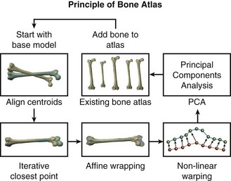
Briefly, a bone atlas is an average mold, or template mesh, that captures the primary shape variation of a bone and allows for the comparison of global shape differences between groups or populations. Bone atlases were developed initially for automatic medical image segmentation2,3,6,13; however, they can be used as a way to digitally re-create a bone and conduct statistical shape analyses.9,11–13 In addition, they have proven useful in biologic anthropology as a means of studying sexual dimorphism, reconstructing hominid fossils, and making shape comparisons among fossil species.9–11,14,17
For the ethnicity difference analysis in this study, a previously developed technique for creating a statistical representation of bone shape was used in a novel manner.9,11,12 Two separate statistical atlases of femora were compiled; one atlas contains only American white femora and the other only American black femora. Likewise, two separate atlases were created for the tibiae and were divided in the same manner (i.e., American white and black tibiae). The processes involved in creating these statistical atlases and adding bones to the atlases are outlined in the following paragraphs.
First, all bone models in the dataset were compared, and a bone model with average shape characteristics was selected to act as a template mesh. The points in the template mesh were then matched to corresponding points in all other training models. This ensured that all bones had the same number of vertices and the same triangular connectivity.12 Next, a series of registration and warping techniques were used to select corresponding points on all other bone models in the training set. This process of picking point correspondences on new models to be added to the atlas is “nontrivial.”9 The matching algorithm described here uses several well-known techniques of computer vision, as well as a novel contribution for final surface alignment.
During the first step in the matching algorithm, the centroids of the template mesh and the new mesh are aligned, and the template mesh is pre-scaled to match the bounding box dimensions of the new mesh. Second, rigid alignment of the template mesh to the new mesh is performed using a standard vertex-to-vertex iterative closest point (ICP) algorithm. Third, after rigid alignment, a general affine transformation is performed without iteration. This method is applied to align the template mesh with the new mesh using 12 degrees of freedom (rotations, translations, scaling, and shear). After the affine transformation step, the template and the new model have reached the limits of linear transformation, but local portions of the models remain significantly distant. Because the goal of final surface-to-surface matching is to create new points on the surface of the new model that will have similar local spatial characteristics as the template model, a novel nonlinear iterative warping approach was developed to reduce misalignment.9
To achieve point correspondence (Fig. 12-1), an iterative algorithm is used where the closest vertex-to-vertex correspondences are found from the template to the new model as before, but now we also find correspondences from the new model to the template model. Using both of these point correspondences, points on the template mesh are moved toward locations on the new mesh using nonsymmetrical weighting of the vectors of correspondence. Next, a subroutine consisting of an iterative smoothing algorithm is applied to the now deformed template mesh. This smoothing algorithm seeks to average the size of adjacent triangles on the template mesh, thereby eliminating discontinuities. At the beginning of the warping algorithm, the smoothing algorithm uses the actual areas of surrounding triangles to dictate the smoothing vector applied to each point; this helps to effectively remove outlying points with large triangles. Consequently, at the beginning of the process, the template mesh makes large steps, and larger smoothing is required. Toward the end of the process, however, the smoothing vector is normalized by the total area of the surrounding triangles, which allows for greater expansion of the template mesh into areas of high curvature. After this procedure has been completed on all the femora and tibiae in their respective atlases, the atlases are ready for morphologic shape analyses and automated metric comparisons.
Automated Measurements
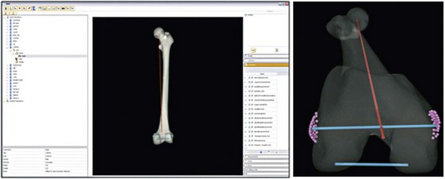
A wide array of comparisons was made using specific measurements at defined landmarks on the ethnicity-specific statistical atlases. These landmarks were chosen on the basis of surgical importance, clinical relevance, and historical measurements. Because the atlas consists of homologous points on each femur (or tibia) model, it provides ample information for automating this process. Also, each bone model in the atlas is aligned with the same coordinate frame. A total of 99 femur and 23 tibia measurements, angles, and indices were calculated, although only a select subset of these variables is defined here. Furthermore, for purposes of concision, only the most significant metric properties are discussed in the results section. Unless otherwise specified, the measurements outlined below represent three-dimensional (3D) Euclidean distances between pairs of landmarks, and angles are measured as 3D rotations between vectors. In some instances, these measurements were projected onto a plane for comparison with previous work in the field. A subset of these measurements is shown in Figures 12-2 through 12-4. Landmarks that define the measurement endpoints are computed and then are defined relative to surgical and anatomic axes.
Stay updated, free articles. Join our Telegram channel

Full access? Get Clinical Tree


