Determination of Component Orientation and Position in Patients After Total Knee Replacement

Fig. 29.1

AP radiograph showing (a) mechanical and (b) anatomical alignment and (c) weight-bearing axis

[

Table 29.1

Differences, pros and cons between the mechanical and anatomical axes of the tibia and femur

	Difference	Pros	Cons
Mechanical axis of the femur	Line from the centre of femoral head to distal femur	1. Easier to appreciate varus/valgus deformity	1. Loss of Whiteside’s and posterior referencing after TKR (affects distal reference points on 3D CT)
Anatomical axis of the femur	Line through 3 mid-shaft points	1. Basis of intramedullary guides used operatively	1. Greater sampling error in using 3 points
		2. Useful when reference points for mechanical axis disrupted, e.g. fracture, slipped upper femoral epiphysis (SUFE)	2. Extra-articular deformity negates use of axis
			3. Dorsal curvature on lateral view makes measurement more difficult
Mechanical axis of the tibia	Line from proximal tibia to mid-tibial plafond	1. Easier to appreciate varus/valgus deformity	1. Loss of proximal reference points after TKR (tibial spines) makes definition more difficult
Anatomical axis of the femur	Line through 3 mid-shaft points	1. Basis of intramedullary guides used operatively	1. Greater sampling error in using 3 points
Anatomical axis of the femur	Line through 3 mid-shaft points	2. Useful when reference points for mechanical axis disrupted	2. Extra-articular deformity negates use of axis

9].

A “true” anteroposterior (AP) view allows evaluation of the varus/valgus of the femoral and tibial components and tibiofemoral alignment (Fig. 29.2).

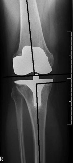
Fig. 29.2

AP radiograph TKR showing measurements: femoral component varus/valgus, tibial component varus/valgus

The standard lateral view of the knee is needed to measure the posterior slope of the tibial component and flexion/extension of the femoral component; however, long-leg lateral views are seldom performed (Fig. 29.3).

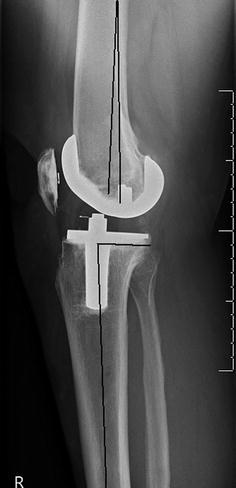
Fig. 29.3

Lateral radiograph showing measurements: femoral component flexion/extension, tibial component posterior slope

Although various methods have been described to measure component axial rotation on plain radiograph [7], this is fraught with a large degree of uncertainty and is increasingly being superseded by CT [5].

Assessment of rotational alignment of the femoral component has been attempted using an axial radiograph of the distal femur, with the knees flexed to 90°. The angle between the clinical epicondylar axis and the posterior condylar axis is measured. This method has been shown to be comparable in terms of reproducibility and correlation with that of 2D CT [10]. Assessment of rotational alignment of the tibial component has been attempted using lateral radiographs of the knee with the knee in full extension [11]. The method requires a component with two tibial pegs, with measurement of the width of the overlapping pegs used as a reflection of component rotation. Although it has been shown to be a useful method, it is limited to certain prostheses, and radiograph quality can markedly alter the results [7].

29.2 Computed Tomography (CT)

29.2.1 Scanning Protocols

There are currently two published and widely used low-dose CT scanning protocols for the postoperative assessment of orientation and positioning of the total knee replacement: the Perth CT protocol [12] and the Imperial CT protocol [13]. The Perth protocol positions the patient supine with both legs in neutral anatomical position, patellae pointing upwards and the knees in maximal extension. Images are acquired over the whole of the lower limb between the superior margin of the acetabulum to the talus with 2.5 mm contiguous slices with a scan time of 40 seconds delivering a radiation dose estimated to be equivalent to 1 year of background radiation. The Imperial CT protocol gives an 80 % reduction in the radiation exposure by limiting the scanned area to only include the whole femoral head, high-resolution 1 mm collimations over the 20 cm at the knee and 5 cm at the ankle. Imaging these three anatomically discrete regions enables the surgeon to define the mechanical axis of the femur and tibia, although it limits the use of the femoral anatomical axis.

29.2.2 2D CT

Two-dimensional (2D) CT can be used to determine component rotation with reference to an anatomical axis. Femoral component rotation can be measured on an axial CT slice as the angle between a line connecting the surgical epicondylar axis and the posterior axis of the component [14] (Fig. 29.4). Tibial component rotation can be measured on an axial CT slice as the angle between a line connecting the posterior condylar axis and the posterior axis of the component [15] (Fig. 29.5).

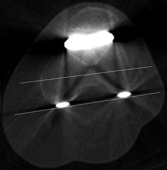
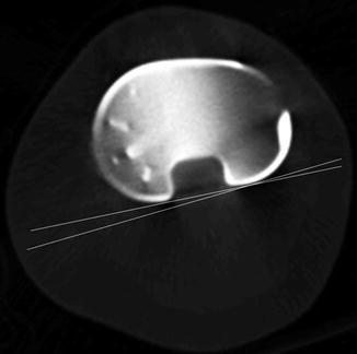
Fig. 29.4

Rotational alignment of femoral TKR component on 2D CT

Fig. 29.5

Rotational alignment of tibial TKR component on 2D CT

The CT scout film is also frequently used to determine limb alignment, however, this should be used cautiously as it has been reported to underdetect malalignment due to it being a non-weight-bearing modality (Fig. 29.6) [16].

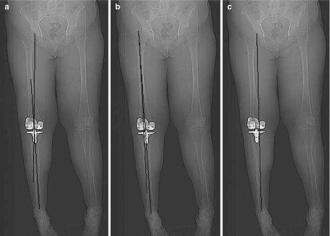
Fig. 29.6

Image of scout film showing (a) mechanical and (b) anatomical alignment and (c) weight-bearing axis

29.2.3 3D CT

Three-dimensional (3D) CT is now becoming recognised as the investigation of choice for the poorly functioning TKR when component positioning is being questioned, as it is more accurate and reliable than 2D CT or conventional radiography in determining component orientation and positioning [5].

29.2.3.1 Extended CT Scale

The use of metal artefact reduction strategies including utilisation of the extended CT Hounsfield Scale available on many CT scanners allows clear visualisation of the metal implants [17] and enables isolation of the prosthetic components with accurate delineation of their surfaces for landmarking and measurement (Figs. 29.7 and 29.8).

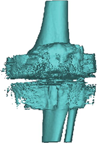
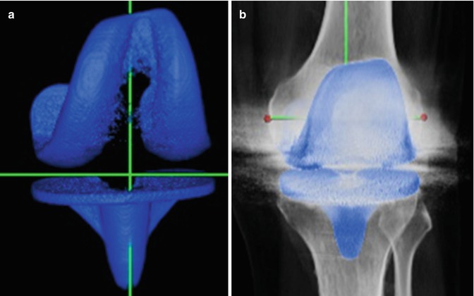
Fig. 29.7

3D CT of total knee replacement without metal artefact suppression sequence

Fig. 29.8

Example of effect of metal artefact suppression sequence (a) Isolated TKR components (b) Isolated TKR components superimposed upon CT

29.2.3.2 Measurement Methods

Conventional radiographs necessitate the radiographer to suitably position the patient to obtain true anteroposterior and lateral views in order to allow reproducible measurements [4].

Although the same principle applies to measurement made on CT, with the reference axes first defined and the images aligned, the three-dimensional nature of the images allows post-imaging reconstruction in all planes and therefore is less subject to positioning “errors”.

29.2.3.3 Femoral Axes

Two longitudinal frames of references (FoR) are widely used for the femur: the anatomical and mechanical axes.

The anatomical axis can be defined using 3–4 bony landmarks in the middle of the femoral diaphysis or alternatively with a proximal point in the piriformis fossa and a distal point in the centre of the distal femur [18].

Only gold members can continue reading. Log In or Register to continue