Chapter 5 Knee Imaging Techniques and Normal Anatomy
Radiography
Applications
Radiographs are the workhorse of knee imaging. Nearly any symptom or sign may be initially evaluated with an x-ray. Radiographs provide useful information across the entire spectrum of knee pathology, including congenital deformities, arthritis, trauma, oncology, sports injuries, metabolic disease, and arthroplasty evaluation.36
Radiographic Views
Anteroposterior Radiograph
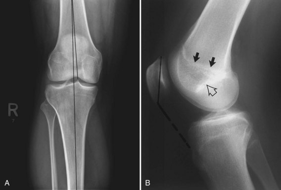
The AP view is obtained with the knee extended, the cassette behind the knee, and the central x-ray beam perpendicular to the cassette. A standing (weight-bearing) AP radiograph more accurately assesses the joint space than one obtained with the patient supine.1,2,31,38 For this reason, as well as to allow the estimation of valgus or varus angulation, weight-bearing images are preferable whenever possible (Fig. 5-1). Normal structures evaluated on every AP radiograph of the knee are the patella, the medial and lateral femoral condyles, the medial and lateral joint compartments, the tibial spines, the medial and lateral tibial plateaus, and the fibula. The AP view also provides a gross assessment of femoral tibial alignment (Fig. 5-2A). The lateral compartment is normally slightly wider than the medial.
Lateral Radiograph
The lateral view is obtained with the knee flexed 30 degrees and the patient lying on the affected limb. The cassette is positioned under the lateral side of the knee, and the x-ray beam is directed perpendicular to the cassette. This view depicts the quadriceps tendon, the patella, the patellar tendons, the suprapatellar bursa, the distal femur, the proximal tibia, and the proximal fibula (Fig. 5-2B).
The medial femoral condyle is slightly larger than the lateral condyle. The lateral femoral condyle can be identified by the presence of the lateral femoral sulcus at the anterior aspect of its weight-bearing portion.34 Blumensaat’s line represents the roof of the intercondylar notch. The closed physeal scar is also evident on the lateral view, and the patella should fall between it and Blumensaat’s line.
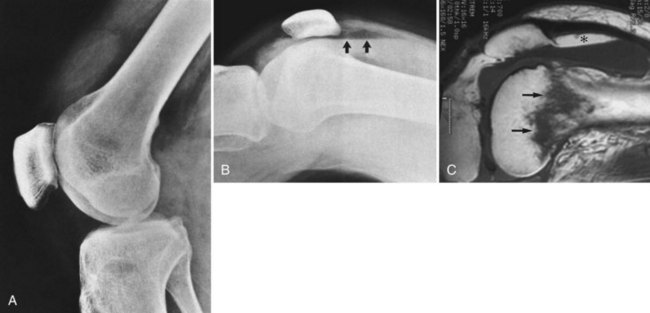
In the setting of a joint effusion and suspected occult intra-articular fracture, a cross-table lateral view is useful for evaluating for lipohemarthrosis. The view is obtained with the patient supine and the knee slightly elevated. The cassette is placed adjacent to the medial knee. This positioning, in contrast to the standard lateral view, is better tolerated by a traumatized patient. The presence of a fat fluid level indicates an intra-articular fracture (most commonly, the tibial plateau) and prompts further evaluation with computed tomography (CT) or magnetic resonance imaging (MRI) (Fig. 5-3A, B, and C).
Superoinferior positioning of the patella may be evaluated using the Insall-Salvati ratio. This is the ratio of the greatest length of the patella divided by the length of the patellar tendon. This ratio averages 1.17 and normally falls between 0.8 and 1.2 (see Fig. 5-2B). A long patellar tendon generates a ratio greater than 1.3, indicating a high patella (patella alta). Conversely, a short tendon accompanies a low patella and a ratio less than 0.8, termed patella baja.
Axial View
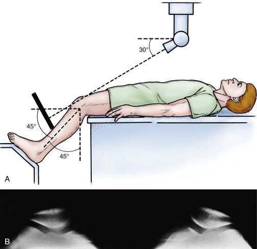
The axial view of choice is the Merchant view.15,35,37 The patient is placed in the supine position on the radiography table; the knees are flexed 45 degrees (using a fixed or adjustable platform), and the cassette is placed on the proximal part of the shins. Both knees are exposed simultaneously, with the x-ray beam directed toward the feet, inclined 30 degrees from the horizontal (Fig. 5-4A). This view provides an excellent assessment of patellofemoral alignment and is ideal for assessing the osseous patellofemoral articular surfaces (Fig. 5-4B). In contrast, a skyline (or sunrise) view is obtained with the patient prone and the knee in maximum flexion. This view demonstrates the posterior surface of the patella and the anterior surface of the femur, but the imaged femoral surface is not at the patellofemoral joint. Furthermore, accurate assessment of patellofemoral alignment is limited when the knee is flexed excessively.7,15 Some patients have difficulty tolerating this position.
Supplemental Views
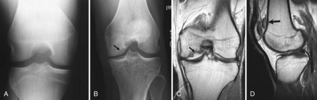
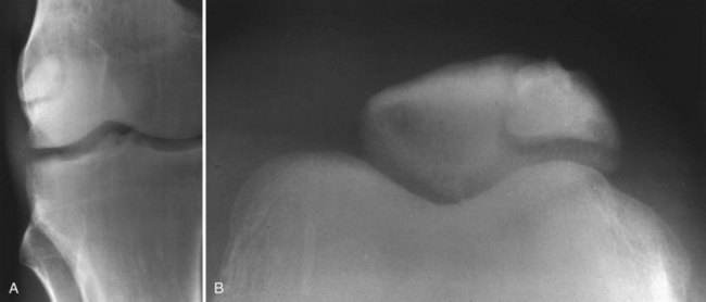
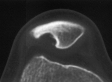
The tunnel view is a frontal view obtained with the knee flexed 60 degrees. It can be obtained AP with the patient in the supine position, or posteroanterior (PA) with the patient prone or kneeling on the cassette. The x-ray beam is directed perpendicular to the tibia. This view demonstrates the posterior aspect of the intercondylar notch, the inner posterior aspects of the medial and lateral femoral condyles, and the tibial spines and plateaus (Fig. 5-5A). It is ideal for evaluating patients with suspected osteochondritis dissecans (OCD), which tends to occur more posteriorly in the intercondylar notch (Fig. 5-5B, C, and D).
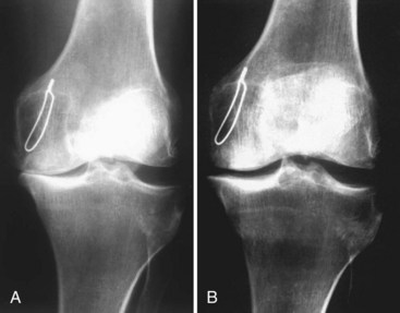
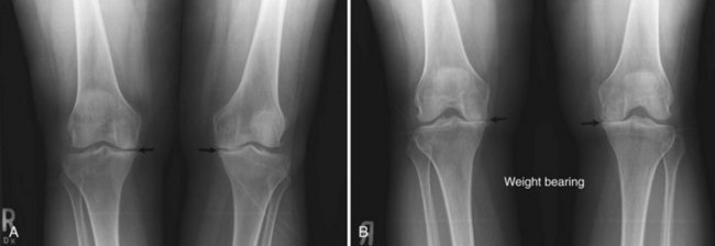
The flexed, PA weight-bearing (Rosenberg) view is a modified tunnel view. It is obtained with the patient standing and the knee flexed 45 degrees. The patellae should touch the film cassette. The x-ray beam is centered at the level of the inferior pole of the patella and is directed 10 degrees caudad. It captures the joint space at the posterior aspect of the femorotibial joint. This view is valuable for evaluating arthritis. It detects joint space narrowing due to cartilage loss that often goes unappreciated or underestimated on a conventional AP weight-bearing view (Fig. 5-6A and B).8,9,25,47,49 Comparisons of intraoperative and radiographic findings demonstrate that the flexed PA weight-bearing view has greater accuracy, sensitivity, and specificity than the conventional extension weight-bearing radiograph.49
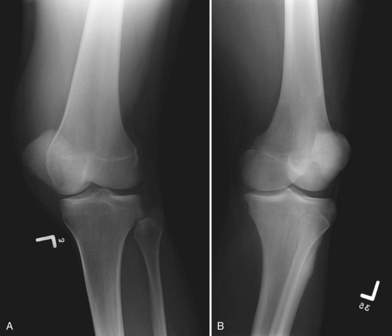
Oblique radiographs complement a routine examination. Occult fractures and tibiofibular arthritis may be more easily detected with oblique views than with routine AP radiographs. Bilateral oblique views are obtained at 45 degrees of internal and external rotation, with the patient supine, the affected knee extended, and the cassette behind the knee. The x-ray beam should be directed 5 degrees cephalad. Views should demonstrate the patella, the femoral condyles, the tibial plateaus, and the fibula. In external rotation, the tibia and fibula are superimposed on each other. With internal rotation, there is less superimposition between the tibia and fibula (Fig. 5-7A and B).
Special Considerations and Anatomic Variants
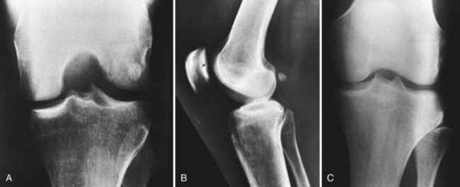
Two sesamoid bones commonly identified on knee radiographs are the fabella and the cyamella. The fabella is located within the lateral head of the gastrocnemius. It overlies the lateral femoral condyle on the frontal view and sits posterior to the distal femur on the lateral view. The cyamella lives within the popliteus tendon. On a frontal radiograph, it may be found at the insertion of the popliteus in the notch of the lateral femoral condyle (Fig. 5-8A, B, and C).
Normal variants also occur in the patella, which can have two or more osseous centers, referred to as a bipartite or multipartite patella (Fig. 5-9A and B). A bipartite patella is the more common variant, seen in 1% of the population. It is bilateral 50% of the time.35 The smaller pieces of the patella are located superolaterally and should fit neatly together like pieces of a jigsaw puzzle. The width of a bipartite patella is usually greater than that of the contralateral patella when assessed on a tangential axial view. MRI depicts intact cartilage overlying a bipartite patella, whereas a fracture displays disrupted osteochondral integrity. These features help dismiss the suspicion of a fracture.35 Rarely (<2% of the time), a bipartite patella can be symptomatic. MRI of the knee may demonstrate bone marrow edema on one or both sides of the synchondrosis.
A dorsal defect of the patella is another anatomic variant, usually detected incidentally. It appears as a lucent area of the superolateral patella (Fig. 5-10).18,26 Pathologically, the lesion is composed of fibrous tissue and spicules of bone. This uncommon entity is seen in children and typically fills in with normal or sclerotic bone in adulthood.
Patellofemoral Alignment
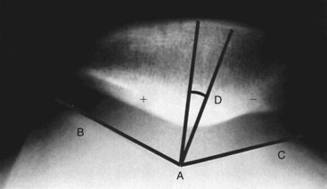
Merchant views can evaluate patellofemoral malalignment, which can be quantified with the sulcus and congruence angles. The sulcus angle is formed by drawing lines outward from the deepest portion of the trochlear sulcus to the tops of the femoral condyles. The angle normally measures 138 degrees (±6 degrees).20 A shallow sulcus greater than 144 degrees is associated with recurrent patellar dislocation.
The congruence angle provides an index of subluxation. To measure it, the sulcus angle is bisected to create a reference line. An additional line is then drawn from the deepest portion of the trochlear sulcus to the patellar apex. The angle formed between this line and the reference line is the congruence angle. If the patellar apex falls lateral to the reference line, then the value of the congruence angle is positive. If the apex falls medial to the reference line, then the value of the congruence angle is negative. The normal congruence angle is six degrees (±11 degrees) (Fig. 5-11).20,37
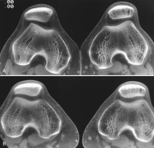
Patellar tilt is another measure of patellofemoral alignment. It is measured by the angle formed between a horizontal line and a line drawn between the medial and lateral corners of the patella. In the study performed by Grelsamer and colleagues, the mean tilt angle of a group of patients with signs and symptoms suggesting patellofemoral malalignment was 12 degrees (±6 degrees); in a similar group of control subjects, it was 2 degrees (±2 degrees). Tilting of 5 degrees was taken to be the limit of normal. It is noteworthy that in the Grelsamer study, the knee was held in 30 degrees of flexion, rather than 45 degrees of flexion in the normal Merchant view.21 Other imaging techniques (CT scans performed at various degrees of flexion) are sometimes necessary to detect patients with subtle or transient lateral patellar subluxation (Fig. 5-12A and B).
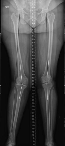
Short- versus Long-standing Views
Obtaining long-standing radiographs requires a long cassette. If a long cassette is not available, a CT scanogram can be obtained. CT scanning to obtain the mechanical axis is not advocated by the authors because it is not weight bearing, does not provide functional information, and may fail to take account of ligamentous laxity. Also, CT scanograms entail higher radiation dosage exposure compared with conventional radiographs (Fig. 5-13).
Arthrography
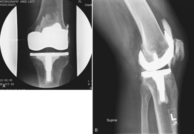
Radiographic arthrography entails intra-articular injection of x-ray dye, typically an iodine-based product. Arthrography has many uses, including confirming placement before joint aspiration. Commonly, once radiographs confirm dye placement within the joint space, a CT or MRI is performed to better evaluate meniscal or articular cartilage pathology and or component loosening (Fig. 5-14).
Computed Tomography
Applications
Computed tomography (CT) provides detailed information about osseous structures and generally functions as a problem-solving modality once the limits of radiography have been reached. Specialized knee applications include evaluation of complex trauma such as tibial plateau fractures, fracture healing, and joint loose bodies. CT is utilized with increasing frequency for preoperative joint replacement planning, arthroplasty complications, and revision arthroplasty preparation.10,29,33,46 Extensor mechanism and patellofemoral joint evaluation in the setting of knee pain has also been reported.22,27,28,32
CT arthrography may be requested to evaluate menisci and/or articular cartilage when a patient is unable to undergo an MRI. This situation is commonly encountered in patients with claustrophobia or MRI-contraindicated metallic devices such as pacemakers.41,58
Technique
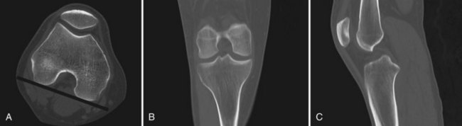
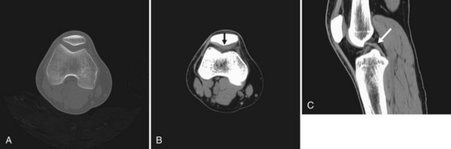
Practically, the knee is imaged axially with thin sections (1.25 or 0.625 mm). The coronal reformats are prescribed via a line connecting the posterior aspects of the femoral condyles. The sagittal plane is generated along a line perpendicular to the coronal plane (Fig. 5-15A, B, and C).
Several techniques are available for reducing metal-related artifact. First off, patient positioning is important. When possible, the goal is to position the patient so the beam penetrates the smallest cross-sectional area of metal. The high density of metal is challenging for a CT scanner because it prohibits the passage of photons. This may be partially overcome by increasing the peak kilovoltage (kVp) and milliampere seconds (mAs). kVp is the maximum voltage applied across an x-ray tube. A higher voltage results in higher energy photons, which possess greater penetrating power. mAs is the quantity of photons produced by the x-ray tube. Raising the mAs means that more photons are available to penetrate the metal and contribute to the image. The pitch may be decreased, typically to less than one, to increase the overlap of slices (think of a tight spiral). This effectively increases the number of image-generating photons. The tradeoff in increasing each of these parameters is increased radiation exposure to the patient. During postprocessing, choosing thicker sections reduces image noise, combating metal-related artifact. Also, because bone algorithms worsen artifact, utilizing a standard reconstruction filter is preferable (Fig. 5-16).
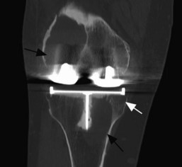
Image Interpretation
A knee CT scan is read in any of three standard imaging planes: axial, sagittal, or coronal. An advantage of a PACS environment is that images can be instantaneously adjusted to focus on a specific range of densities to best show the tissue(s) of interest. A center density is identified, termed the level. The second setting, the window, is the range of densities around the level. For example, to evaluate fine bony detail, a level of 500 HU and a window of 2000 HU might be elected. In contrast, to assess soft tissue structures such as the menisci or cruciate ligaments, a level of 40 HU and a window of 400 may be chosen. These different bone and soft tissue settings are often programmed into the PACS and can be quickly selected at the touch of a button (Fig. 5-17A, B, and C).
Related posts:
 Cemented Total Knee Arthroplasty: The Gold Standard
 Management of Extra-articular Deformity in Total Knee Arthroplasty With Navigation
 Patellar Instability
 Posterior Cruciate Ligament Reconstruction: Posterior Inlay Technique
 Anterior Cruciate Ligament Reconstruction With Central Quadriceps Free Tendon Graft
 Osteochondritis Dissecans
Stay updated, free articles. Join our Telegram channel

Full access? Get Clinical Tree


