Review of Statistical Approaches for the Analysis of Data in Rheumatology
where Xirepresents here the DAS28 value for the ith patient and n = 159 is the size of the RAPPORT study. The symbol signifies that the sum is taken of all 159 patients of the RAPPORT study. In contrast, HAQ has a right-skewed distribution (with a right tail). The median value corresponds to the value such that 50 % of the observations are left to it; it is also referred to as the 50 %-ile and denoted as Q50. While the median can always be interpreted as a central value, this is not necessarily the case for the mean value, see, e.g., Fig. 1b for HAQ. The spread of the collected data around a central value can be expressed in various ways. The standard deviation (denoted as s or SD) is the square root of the variance s2, which is equal to the average squared deviation of the data from their mean, i.e., . The SD has the advantage over the variance that it is expressed in the original units of the data. For example, since blood pressure is measured in mmHg, the variance is expressed in mmHg2, while the SD is also expressed in mmHg.
Fig. 1
RAPPORT study: (a) histogram of DAS28 at baseline together with the best fitting normal distribution, (b) histogram of HAQ at baseline together with the best fitting normal distribution, (c) box plots of DAS28 and HAQ at baseline, and (d) error bar plots of DAS28 and HAQ at baseline. The histograms have the property that the total area of the bars is equal to one. M represents the mean and m represents the median. In the error bar plots, the longest bars have length equal to the standard deviation; the shortest bars represent the SEM
When the SD is greater in treatment arm A than in arm B, we conclude that the variability of the data must be greater in A than in B. However, apart from this interpretation, it is not immediately obvious how the SD relates to the spread of the data. An alternative, easier-to-interpret, measure is the interquartile range (IQR), defined as Q75 – Q25, where Q25 is the 25 %-ile and Q75 is the 75 %-ile of the data. The IQR is therefore easily understood as the length of the central interval that contains 50 % of the data. The mean and median are called summary statistics for location, while SD and IQR summarize the variability of the data. The mean/median (SD/IQR) for DAS28 in Fig. 1a is 3.37/3.28 (SD = 1.31/ IQR = 3.28 − 2.42 = 0.86), while for HAQ (Fig. 1b) we have 0.62/0.50 (SD = 0.63/IQR = 1.00 − 0.125 = 0.875).
It is customary to summarize continuous data in medical publications with mean ± SD. While not always understood, this tradition stems from assuming that the interval [mean-SD, mean + SD] contains 68 % of the central data. However, this interpretation only holds when the histogram can be well approximated by the Gauss curve or distribution. The Gauss distribution, also called the “normal” distribution, is the most used distribution in mathematics and statistics, see, e.g., [4, 5]. It reflects the stochastic behavior of a random measure that is the result of the sum of many independent causative factors. Typical measurements that have a normal distribution in a general population are height and weight. For DAS28 the interval [3.37 − 1.31, 3.37 + 1.31] contains indeed 68 % of the central data. The 68 % CI for HAQ, equal to [0.62 − 0.63, 0.62 + 0.63], contains about 80 % of the data, but more importantly it contains negative values, which is clearly nonsense. In Fig. 1, we observe that the Gauss curve approximates well the histogram of DAS28, but not for HAQ.
The error bar plot is a popular way to graphically represent the characteristics of the data. In Fig. 1d we show this plot for DAS28 and HAQ. The height of the rectangle is equal to the mean, while the bar emanating from it has length equal to the SD. Hence, this plot graphically displays the interval [mean, mean + SD]. While popular, this plot cannot reveal a possibly skewed distribution of the data. An alternative graph is the box (−whisker) plot shown in Fig. 1c. The edges of the box represent Q25 (lower edge) and Q75 (upper edge); the horizontal line represents the median. The lines emanating from the box are called whiskers. The whiskers give a graphical impression of the skewness of the distribution. The dots indicate outlying values. The definition of the whiskers and outliers depend on the software (here, R).
Time–to–event data express the time until the event of interest occurs. This event includes, besides death, also nonterminal events such as remission (DAS < 1.6) in an RA study, a cardiac event in a cardiology study, caries in a dental study, etc. Another term for such data is survival time. Typically, survival times have a (right) skewed distribution, and hence the median (and IQR) is here preferred over the mean (and SD). However, most often the exact survival time is not known but is censored. A survival time is right censored when it is only known that the event hasn’t happened during the conduct of the study. Left censoring occurs when event happened before the patient entered the study. This may occur in retrospective studies but such patients are excluded in cohort studies where an association between a risk factor and the event is examined. Interval censoring is relatively common in clinical studies. A survival time is interval censored when it is only known that the event has occurred between two examinations. In this chapter we consider only right censoring. There are various reasons for (right) censoring. For instance, when patients are recruited rather late in the study, the probability is low that they will experience the event. Other reasons are: a patient leaves the study prior to experiencing the event because he changed medication, because of adverse events, because the patient died, etc. It is important to mention that the time at which censoring occurs must not be correlated with the survival time. For instance, removing patients from the study immediately prior to experiencing an event will bias the results and the conclusions of every survival analysis applied to the time-to-event data.
Classical statistical descriptive and inference techniques are not appropriate for survival data. Indeed, for a right-censored survival time, the true survival is only known to be greater than its recorded value. Hence, the mean (median, SD, histogram, box plot, etc.) of the recorded (censored) survival times cannot provide a good estimate of the mean (median, etc.) of the true survival times. Indeed, dedicated techniques are needed in such a case, such as the Kaplan–Meier curve. This curve is a proper estimate of the distribution of the true survival times, called the survivor function. In Fig. 2, we show the Kaplan–Meier curve of a fictive RA study where RA patients were followed up from the first time they were in remission until their DAS increased above 1.6. This curve shows for each possible survival time (less than the maximum observed time) the estimated proportion of subjects in remission. The Kaplan–Meier curve provides also an estimate of the median survival time, which here is 1.5 months; see Fig. 2. However, the Kaplan–Meier curve cannot provide other descriptive statistics such as the mean survival and its SD. Note that, in the fictive RA study, we assumed right censoring, while in practice, interval censoring certainly would apply since DAS needs to be determined at examination times by the treating rheumatologist.
Fig. 2
Fictive study: Kaplan–Meier curve that estimates for each time point the proportion of patients that are still in remission. The symbol “+” indicates when the “survival” time is right censored. The arrow points to the estimated median “survival” time. The dashed lines correspond to the 95 % CIs at each observed time of “death”
Introduction to Statistical Inference
The Sample and the Population
The goal of drug research is to establish the effect of an experimental medication for all possible eligible patients. These patients constitute the population. The population of subjects for whom the drug may apply is to some extent artificial since some of the eligible patients may not have been born yet. For this reason, but also due to practical (financial, time constraints, etc.) considerations, it is almost never possible to examine the whole population of interest, and one must confine to a limited set of subjects.
When the sample is taken in a random manner from the population, probability laws can tell us how the sample characteristics vary around the population characteristics. For instance, when a new DMARD reduces DAS28 after 3 months on the average with 0.5, then this average will fluctuate from study to study around its true mean μ (=0.5). The variability in the study mean is expressed by the standard error of the mean (SEM). It is in principle impossible to know SEM since studies are never repeated in exactly the same way. However, from probability laws, we know that it can be estimated from a single study using the formula . This formula shows that when the patient population is homogeneous (small variance) and/or the study is large, there is little variation of the sample mean around the true mean and then taking the study mean for the population mean will not induce a great error. One can also guess the distance between the true and sample mean with the confidence interval (CI). Namely, the 95 % confidence interval given by contains the true mean with 0.95 probability. Note that the coefficient “2” in the above expression is approximate and varies with the study size, as seen later. Thus, the smaller the 95 % CI, the more precise statement we can make about the true mean. For the RAPPORT study, the SEM of the mean DAS28 at baseline is equal to (for some patients, DAS28 is missing), yielding a 95 % CI equal to [3.15, 3.58]. This implies that we are not sure about the true mean of DAS28, but we believe with 95 % certainty that it is greater than 3.15 and smaller than 3.58. For HAQ at baseline, we obtained an and the 95 % CI now becomes [0.52, 0.72]. Bars have been added in Fig. 1 that represent the SEM.
Finally, note that the 95 % CI is most popular, but confidence intervals of any size can be determined. In fact, occasionally one reports the 90 % CI or the 99 % CI.
The above probability properties hold when the sample is taken from the population by random sampling (simple random sampling or a more sophisticated version) mechanism. This is often not possible but rather a convenience sample is taken, as with the RAPPORT study. This is a sample that is obtained by simply collecting the information from (consecutive) patients who are available to the investigator. The problem with a convenience sample is that it is not obvious how the results can be extrapolated to a well-defined population. A similar problem occurs with randomized clinical trials (see chapter “The randomized controlled trial: methodological perspectives”).
Basic Tools for Statistical Inference
Statistical inference is the activity to draw conclusions from subjects examined in an experimental or observational study for use in future similar subjects. For example, in the RAPPORT study, we might be interested to know whether the change in average DAS28 (in a 12 months’ period) differs between men and women. The average difference (DAS28 at 12 months – DAS28 at baseline) for the 26 men for whom both measurements were recorded is equal to 0.10 (so in fact an increase in disease activity was noticed) and it is −0.052 for the 81 women. The difference in averages is not equal to zero. But our interest lies in the difference of means between men and women for the populations from which the RAPPORT patients were taken, i.e., in the difference between μmale and μfemale. The 95 % CI of μfemale − μmale, computed from the patients with a recorded DAS28 value at both examinations, is equal to [−0.69, 0.38]. This interval expresses what we know about the true difference from the patients in the RAPPORT study. Since this interval includes zero, we cannot rule out a zero difference in the true means and we decide that there is no (strong) evidence of a different mean change in DAS28 after 12 months of treatment between men and women. Suppose now that we wish to know whether the mean age of women in the RAPPORT study is different from that of men. The mean age of the 121 women is 51.5 years, while for the 38 men, it is 58.4 years. Again we compute the 95 % CI of μfemale − μmale, where μ now represents the average age, and obtain [−11.60, −2.08] (in years). Now the interval excludes zero; hence, we conclude that there is (strong) evidence that on average women are younger than men in the RAPPORT population.
The confidence interval provides a direct way to draw inference from the study to the population. Yet, a more popular and indirect way of inference is based on the P–value. When comparing two (unknown true) means, μ1 and μ2, one can distinguish two hypotheses:
The hypothesis of interest is given by Ha, called the alternative hypothesis. To test this hypothesis, one reasons indirectly and questions whether H0, called the null hypothesis, can be rejected. This is done via the P-value. To establish the P-value, one computes the difference of the two observed means and evaluates the extremeness of this difference if Δ = 0 were true. The P-value is the result of a statistical test and expresses the probability that the observed difference (or more extreme) could have been obtained under H0. A P-value is sometimes referred to as a surprise index. When the P-value is small, doubt is raised about H0 and one is inclined to reject it. Classically a P-value less than 0.05 or less than 0.01 is considered a value too small to sustain the null hypothesis. When P < 0.05, one says that the result is statistically significant at 0.05; when P ≥ 0.05, a nonsignificant result is obtained. The value of 0.05 is called the significance level of the test (in statistical handbooks denoted as α = 0.05). The significance level needs to be chosen prior to performing the computations. In this chapter we consider only α = 0.05, which is the most popular choice but there is in principle nothing against choosing α = 0.01 or α = 0.10, or any other value as long as the significance level is specified prior to performing the test. The average decrease in DAS28 in 1 year’s time between men and women corresponds to P = 0.57, which is not smaller than 0.05, and hence we see no (strong) evidence against H0. The conclusion is then that the two groups are not statistically significantly different at 0.05 (often denoted as NS). On the other hand, for the comparison of the average age between men and women, we find P = 0.0052. This result is now statistically significant at 0.05 (often indicated by *) and we state that H0 is rejected at 0.05.
The statistical test used above is the two–sample t–test, also referred to as the Student’s t–test. The test consists in computing a standardized difference of the two sample means and , i.e., , whereby is the standard error of the difference in means (similar to the SEM of a single mean). This standardized difference T is then compared to a reference distribution, here the t–distribution with (n1 + n2 − 2) degrees of freedom (df). This distribution reflects the natural variability of T under the null hypothesis that Δ = 0. The degrees of freedom is a parameter that depends on the sample sizes of the groups and determines the particular t-distribution. Note that when df ≥30, the t-distribution becomes close to the normal distribution. For the comparison of the change in DAS28 between men and women, df = 26 + 81 − 2 = 105. Under the null hypothesis one expects that T varies around zero, which translates into a statement that under H0 there is 95 % chance that T is located between two extreme values roughly equal to −2 and 2 (which change with df). Observed T values outside this central interval thus indicate that the null hypothesis may not be true and correspond to a P-value smaller than 0.05. For the DAS28 comparison, this interval is equal to [−1.983, 1.983]. We obtained T = −0.577, which belongs to the above central interval and therefore P > 0.05. For the comparison of the mean ages between men and women, df = 157 and the central interval is now [−1.975, 1.975]. Since T = −2.836 does not belong to this interval, P < 0.05.
The two-sample t-test is one of the many statistical tests that were developed over the last century to address the various research questions posed in empirical research. Much of this chapter deals with reviewing a variety of statistical tests. A list of popular statistical tests to compare two groups is given in Table 1 and will be further below discussed in section “Statistical tests to compare two groups.”
Table 1
Overview of classical statistical tests to compare two groups
Type of measurement
Distributional assumptions
Large study
Small study
Unpaired
Continuous
Normal in each group and = variance
Two sample t-test
Two sample t-test
Normal in each group and ≠ variance
Welch test
Welch test
Continuous
Not normal and = variance
Two sample t-test
Wilcoxon rank-sum or Mann–Whitney testa
Not normal and ≠ variance
Welch test
Binary
Chi-square test
Chi-square test + correction
Fisher’s exact test
Paired
Continuous
Difference normally distributed
Paired t-test
Paired t-test
Difference not normally distributed
Paired t-test
Wilcoxon signed-rank testa
Binary
McNemar test
McNemar test + correction
Binomial test
aCan also be used for ordinal data
One-Sided and Two-Sided Confidence Intervals and Tests
The confidence intervals and P-values introduced in the previous section are two sided. For example, in section “The sample and the population,” we have seen that the 95 % CI of the mean DAS28 at baseline is equal to [3.15, 3.58]. This interval is bounded at both sides and contains with 0.95 probability the true value. Further, there is 0.025 probability that the true value is below 3.51 and 0.025 probability that the true value is greater than 3.58. We could, however, also give a one–sided interval like [3.15, infinity]. This interval expresses that there is 97.5 % probability that the true value is above 3.15. Most often, though, a 95 % two-sided interval is reported.
The P-values reported in the section “Basic tools for statistical inference” above are also two sided and therefore sometimes denoted as 2P. When comparing two means, this means that the null hypothesis will be rejected when the standardized difference of means is either too large positively or too large negatively. Often in practice we must be able to reject the null hypothesis for large positive and large negative differences. Let’s take the following example from drug research: A drug company is primarily interested to discover whether their drug is working better than the control drug. In other words, the prime interest lies in rejecting a difference in favor of the experimental drug. Suppose that in a large study, the standardized difference is equal to 1.69 (value obtained from standard normal table) in favor of the experimental drug. Since under the null hypothesis of equal treatment effects, 5 % of the studies show a better result than 1.68, the one-sided P-value is smaller than 0.05. But the threshold for two-sided significance is 1.96, and hence at a two-sided level of 0.05, the result is not significant at 0.05. “One-sided” means that we look only in one direction, here in the direction of a better result for the experimental treatment. On the other hand, suppose that the standardized difference is equal to −3, then the two-sided P-value is smaller than 0.01 pointing toward a worse effect of the experimental treatment. However, the one-sided P-value in the direction of a beneficial effect of the experimental treatment is greater than 0.999. While there is no evidence for a significantly better result for the experimental treatment, there is also no evidence for a worse effect with the one-sided test because one looks away from worse experimental results. Therefore, regulatory agencies demand to use two-sided tests (except for non-inferiority tests, see chapter “The randomized controlled trial: methodological perspectives”).
Type I Error, Type II Error, and the Power of a Test
The fundamental problem in empirical research is that one is never sure about the truth. In fact, if the truth were known then empirical research is obsolete and statistical inference is not needed. Hence, it is upfront never clear whether the null or the alternative hypothesis is true so that every decision based on observed data is prone to two errors. The Type I error represents the error when one concludes that the alternative hypothesis is true (e.g., two treatments have a different effect), while the null hypothesis is in fact true (the true treatments have equal effect). But the researcher may also decide that there is no evidence for the alternative hypothesis, while in fact it represents the truth. In the latter case, a Type II error is committed and then the researcher fails to see that the two treatments really differ in efficacy. The Type I error is controlled by the construction of the statistical test. Namely, by choosing a significance level of 0.05, one automatically fixes the probability of the Type I error to 0.05, called Type I error rate. However, the probability of the Type II error is not fixed in advance and depends on, among other things, the study size. The probability of not committing the Type II error is known as the power of the test and is equal to the probability of finding a clinically relevant difference in the two groups, if it exists. Establishing the sample size to achieve a desirable power is a necessity in randomized controlled trials but is also desirable in explorative studies. Such a computation is, however, quite technical (see chapter “The randomized controlled trial: methodological perspectives”).
The above reasoning indicates that statistical inference is based on repeated sampling ideas. That is, the significance level of 0.05 means that the probability of a Type I error is fixed at 0.05. In other words, (even) if the null hypothesis is true then roughly five out of hundred (independent) statistical tests are significant at 0.05. The practical implication is that, when a large number of statistical tests are performed in a study, say that a few hundred of variables are compared between two groups with about 5 % of them statistically significant at 0.05, then, quite likely, the two groups are not different at all (null hypothesis is probably true). Similarly, the power is also expressed in terms of repeated samplings. Namely, when the power is 0.80 for a clinically relevant different effect, say Δa, then we expect in 100 similar studies at least 80 of them with a statistically significant result at 0.05 if the difference is indeed at least Δa. Finally, the technical definition of the 95 % CI is that in 95 % of the studies set up in the same way as the current study, the true population value is included in the 95 % CI. But for the current study, the true value is inside or outside that interval. This approach of statistical inference, called the frequentist approach, is still most popular in clinical research.
In the frequentist approach, the null hypothesis of equality of group means, proportions, etc. can never be demonstrated. Admitted, such a hypothesis never holds in practice (except when two identical treatments are administered). A nonsignificant result must therefore be interpreted as the “absence of evidence against the null hypothesis” possibly due to a too small study size.
The Bayesian approach is an increasingly popular statistical approach for inference but based on quite different principles. In this approach, the role of the P-value is taken over by a probability that the hypothesis of interest is true after having done the experiment, called the posterior probability. This probability addresses, in contrast to the P-value, the research question directly. In section “The Bayesian approach” we will elaborate on this approach.
Choice Between P-Value and Confidence Interval
The analyses of the RAPPORT study in section “Basic tools for statistical inference” show that zero is inside/outside the 95 % CI of a difference in means when the result is not statistically/statistically significant at 0.05. This is true for most statistical tests. We have:
P ≥ 0.05 (<0.05) if and only if the 95 % CI of the difference does (not) include zero.
The 95 % CI is, however, more informative than the P-value since it also provides the uncertainty with which the true effect is estimated. With the P-value, inference is disconnected from the substantive problem and may easily lead to interpretational problems. For instance, there is a long-standing debate in the literature about whether a significant P-value weighs more in a large rather than in a small study [16]. Major clinical journals like the NEJM, the Lancet, etc. now require reporting confidence intervals. For instance, the NEJM guidelines for the authors stipulate: “Measures of uncertainty, such as confidence intervals, should be used consistently, including in figures that present aggregated results.” Nevertheless, the P-value is still here to stand for some time. However, it will probably not be the only basis for statistical inference in the future.
Use and Misuse of the P-Value
The P-value remains the most used but also the most misused tool for statistical inference. For instance, the P-value is often misinterpreted as the probability that the posed hypothesis is correct. This, in fact, is the very probability which clearly interests the researcher most. However, it can only be obtained by the Bayesian approach, as will be seen in section “The Bayesian approach.”
Another quite frequent misuse of the P-value consists in ignoring the increased risk of committing a Type I error when repeatedly testing for significance. This is called the multiple testing problem. An example illustrates the problem. An experimental treatment is compared to a control treatment in two different studies, with a P-value of 0.03 in the first study and a P-value of 0.06 in the second study, both in favor of the experimental arm. With α = 0.05, there is in each study a risk of 5 % to claim that the two treatments are different while they are in fact equally effective. If better performance of the experimental treatment is concluded when at least one of the studies shows a significant result at 0.05, then the total risk under the null hypothesis of committing a Type I error is about 10 % and not 5 %—what we aimed at!
The Bonferroni correction provides an easy but somewhat crude way to deal with the multiple testing problem. For two tests, the Bonferroni correction consists in dividing the significance level by two, i.e., α = 0.5/2 = 0.025. Significance in each test is then claimed only if P < 0.025, reducing the overall risk back to approximately 5 %. In our example the treatments cannot be claimed different in efficacy based on Bonferroni’s correction. For k tests, Bonferroni correction consists in dividing the significance level by k, i.e., α/k. For k large, it will then become hard to claim any result significant at 0.05. Equivalent to Bonferroni’s correction is multiplying the P-value with the number of statistical tests, and check whether the product is lower than α [17]. For example, with 10 tests, 10 × P must be smaller than 0.05 for a test to be called significant at 0.05. In Chapter “The randomized controlled trial: methodological perspectives”, we will treat more refined ways to correct for multiple testing in controlled clinical trials.
There are several versions of the multiple testing problem. Examples are: two treatments compared in several studies (above example), two treatments compared at several time points or for several variables, more than two treatments compared, etc. In (medical) publications, many statistical tests are often needed to arrive at a sound (clinical) conclusion. Correction for multiple testing may not always be an issue, especially for the exploratory part of the study, as long as one is clear about the nature (exploratory) of the tests. A greater concern is opportunistic testing, i.e., searching as long as the tests confirm what you always wanted to prove. This is called data dredging and emerges especially with a lot of data but no available scientific theory. Finally, we note that statistical testing does not always make sense. For instance, a significance test that compares the baseline characteristics of treatments in a randomized controlled trial makes no sense since at the start, the treatment groups are by definition sampled from the same population.
Statistical Tests to Compare Two Groups
Factors That Determine the Choice of the Statistical Test
Table 1 contains common statistical tests to compare two groups of subjects. The choice of the appropriate test depends on many factors and here we consider four factors: (1) paired versus unpaired data, (2) continuous or binary data, (3) small versus large study, and (4) whether distributional assumptions are met or not. Statistical tests for counts are not included in the table since they are often analyzed (after transformation) as continuous data. If needed, the reader can check the statistical literature for more appropriate tests.
Examples of paired data are two measurements taken on the same subject at two time points or sometimes measurements recorded on siblings. This comes down to two groups of related data, where one group contains the first measurements and the other group the second measurements. With unpaired data, there is no (systematic) relationship between the measurements. Two groups of continuous data are most often compared via the difference in means or via whole distributions, depending whether some distributional assumptions are met or not. Two proportions are compared in different ways, depending on the type of study. With two observed proportions p1 and p2, the absolute risk reduction AR is defined as p1 − p2. In epidemiological research, it is more customary to work with the relative risk RR = p2/p1 or the odds ratio.
Another factor is the size of the study. However, we must admit that a general definition of a large study is lacking, since it depends on technical aspects of the statistical test. For instance, two groups of 1,000 subjects certainly qualify for a large study to compare two means, but perhaps not when two proportions of rare events are compared.
Furthermore, in applying certain tests, some distributional assumptions need to be met, like that the data should have a normal distribution or that variances should be equal.
That the choice of a statistical test depends on the above (and even other) conditions is purely technical and depends on probability laws developed under the above-specified conditions; see, e.g., [4, 5]. When the aforementioned conditions are fulfilled, the reported P-value and 95 % CI are correct. But these conditions rarely apply exactly in practice. For instance, data are never exactly normally distributed. Usually simulation studies are conducted to determine the operational characteristics of these tests under deviations from these conditions. This gives us a hint of when the reported P-value and 95 % CI are to be trusted in practice. We say that a statistical test is robust against an assumed condition when the reported P-value is still correct despite this assumption violated by the data; see the section before, and below “Common statistical tests for the comparison of two groups” below for examples.
In addition to the above, still other factors may play a role in choosing a particular test. For instance, if one is concerned about the impact of outliers on the conclusions of a statistical analysis, a test may be needed that is more robust against such outlying values.
In the next section, we review the statistical tests shown in Table 1. This table can be used as guide when performing simple comparisons between two groups or as a tool to understand better the Materials and Methods part of a clinical paper.
Common Statistical Tests for the Comparison of Two Groups
Continuous Data
The t-test introduced in the section “Basic tools for statistical inference” compares the means of, say, two treatments. This test is appropriate for unpaired data from two groups each having a normal distribution with equal variances. For unequal variances but normal distributions, the t–test for unequal variances, also called the Welch test, applies. However, the classical t-test also works well in this case when the group sizes are about the same, called the balanced case. This was discovered via computer simulation studies. The variance of DAS28 at baseline of men and women in the RAPPORT study is equal to 1.50 and 1.17, respectively. Hence, the Welch test seems at its place here, giving P = 0.54, but this is basically the same to what is obtained from the classical t-test. Another condition for the unpaired t-test is normality in each group. Computer simulations have shown that the t-test is robust against non-normality in the balanced case. For extremely skewed distributions, it may be prudent, however, to check the outcome of the t-test with a nonparametric test. Such a test does not depend on the normality assumption. In fact, for a nonparametric test, the data are replaced by their ranks, and hence the P-value from the test becomes independent of the distribution of the data. A popular nonparametric test is the Wilcoxon rank–sum test, also called the Mann–Whitney U test. A small fictive example illustrates how the test works. Suppose that the DAS28 scores after one year of treatment for group A are 1.0, 1.7, 2.9, and 4.5 and for group B are 2.1, 3.1, 3.3, and 5.9. To compute the Wilcoxon statistic, these scores are ranked irrespective of their group assignment, but their group membership is secured. The ordered values are then 1.0, 1.7, 2.1, 2.9, 3.1, 3.3, 4.5, and 5.9 with the underlined scores pertaining to group B. In the next step, these ordered values are replaced by their ranks 1, 2, 3, 4, 5, 6, 7, and 8, and the ranks pertaining to A are added to give the Wilcoxon rank-sum test statistic W = 1 + 3 + 4 + 7 = 15. The extremeness of the obtained W is established using probability laws with a P-value as result. Here P = 0.484 demonstrating that there is no evidence that the treatments differ in efficacy after one year. In addition to robustness of deviations from normality, a nonparametric test is less vulnerable to outlying values. A disadvantage of a nonparametric test is that the link with the original data is broken, providing basically only a P-value. Note that Wilcoxon rank-sum test can also be used for ordinal data.
Another way to deal with non-normal distributions is to transform the original data such that the transformed data have a normal histogram. The logarithmic function is a popular choice for right-skewed data but may not work when there are a lot of ties in the data. For the HAQ score at baseline, 38 patients have a zero score in the RAPPORT study. Before applying the log transform, we added 1 to the score but then the 38 log (HAQ + 1) scores are equal to zero and thus log (HAQ + 1) cannot have a normal distribution. In fact, none of the classical transformations, including the square root, can turn the distribution of HAQ into a normal distribution. Further, in a comparative study, it often happens that a different transformation is needed in each of the groups. In that case, transforming the data is not an option. In addition, an interpretation problem may arise when results are based on transformed data. For instance, when the data are log transformed, the 95 % CI of the difference in the means on log scale translates into a 95 % CI of the ratio of geometric means on the original scale. But such a 95 % CI is more difficult to interpret as the geometric mean is not equal to the classical mean.
In the case of paired data, inference is based on the difference between the two related values. A statistical significant result is obtained when the mean difference is remote from zero, taking into account statistical fluctuations under H0. The classical statistical test is now the paired t–test. This test requires that the difference of the two related values has a normal distribution. If we do not wish to assume this, one could apply the nonparametric Wilcoxon signed–rank test, which is now based on the ranks of the differences. This test is also appropriate for ordinal data.
Nonparametric statistical tests can be applied to all studies regardless of their size. For large studies, the t-test is also applicable even when the data grossly deviate from normality. This is a consequence of The Central Limit Theorem, a key result in statistics which allows working with the original data (of any distribution) for large studies. In practice “large” means in the balanced unpaired case, group sizes of about 20 or more depending on the deviation from normality, but large(r) sample sizes may be needed in the unbalanced case.
Binary Data
When the outcome of interest is binary, the comparison of two groups involves contrasting two proportions. For unpaired data and a large sample size, the recommended test is the chi–square test. This test essentially evaluates a standardized version of the squared difference of the two proportions under the null hypothesis, which is now that the true proportions and πBare equal. Suppose the observed proportions under treatments A and B are given by pA and pB, respectively, then the chi-square test computes X2 = (pA − pB)2/SE(pA − pB)2, with SE(pA − pB) the standard error of the difference in proportions under H0. When X2 is too large (compared to what is expected under the null hypothesis), H0 is rejected (at α = 0.05). For the actual calculation of the P-value, the chi–square distribution with one degree of freedom is used as reference distribution. Table 2 represents a 2 × 2 contingency table contrasting the frequencies of men and women in the RAPPORT study who require step-up treatment (DAS28 > 3.2). This table is a special case of an r × c contingency table when there are r rows and c columns in the table. In Table 2 the lower case symbols stand for the observed frequencies, while the upper case symbols refer to the expected frequencies, i.e., those that one would expect on average to happen under the null hypothesis. Comparing the observed with the expected frequencies leads to an equivalent expression of X2 given by
Table 2
RAPPORT study: observed and expected frequencies of patients split up according to gender who need a more intensive treatment at month 12
Observed
Expected
DAS28 ≤ 3.2
DAS28 > 3.2
DAS28 ≤ 3.2
DAS28 > 3.2
Men
a = 17
b = 11
A = 14.25
B = 13.75
Women
c = 40
d = 44
C = 42.75
D = 41.25
The above expression shows that X2 will be large when the observed frequencies deviate a lot from the expected frequencies. For the data in Table 2, we obtained X2=1.44 which corresponds to a P-value of 0.23.
For a small study, the chi–square test with continuity correction can be used, but Fisher’s Exact test is recommended. Both tests give a more accurate P-value than the chi-square test for a small study. Now “small” is given by the Cochrane conditions, which stipulate that the chi-square test may be used when the expected frequencies all exceed 5 (satisfied in our example). The P-value for the Fisher’s Exact test is equal to 0.28.
Instead of applying the chi-square test, which only provides a P-value, one could also compute the 95 % CI of the absolute risk reduction AR = pA − pB, with pA = b/(a + b) and pB = d/(c + d). When the 95 % CI of AR does not include 0, the two treatments are statistically significantly different at 0.05. For the relative risk and the odds ratio , the value of 1 must not be within the 95 % CI to claim a significant effect. Using the observed frequencies in Table 2, the odds ratio is easily seen to be equal to ad/bc. For the entries in Table 2, we obtained RR = 1.28 with 95 % CI = [0.88, 1.85] and OR = 1.7 with 95 % CI = [0.71, 4.06]. Both intervals do include 1 and hence there is no evidence for a difference in the true proportions between men and women.
For paired binary data, a similar reasoning applies but of course the tests must differ. An example of paired proportions is the proportion of patients that have in the RAPPORT study a DAS28 less than 3.2 or greater than 3.2 at baseline (first proportion) versus this proportion at 12 months (second proportion). For a large study, a McNemar test is appropriate, which is a variation of the classical chi-square test. For a small study, a corrected version is used or the binomial test.
Survival Times
In section “Describing the collected data,” we have introduced survival data and mentioned that censoring complicated the analysis of such data. Only right censoring is considered here, which means that it is only known that the survival time is greater than the one recorded in the study. Figure 2 shows the Kaplan–Meier estimate (+95 % CI) of the survival function. The Kaplan–Meier curve is a nonparametric estimate, i.e., no assumption is made about the distribution of the true survival times. If one is willing to assume that the survival times have, say, a Weibull or a lognormal distribution, then estimates of the mean survival time, its SD, etc. can be derived. However, in survival analysis, there for no generally accepted distribution. Therefore, one is reluctant to base inference on a particular parametric assumption.
We will defer statistical inference with survival data to section “Cox regression,” where the Cox proportional hazards (PH) model is introduced. For now, we will limit ourselves by mentioning that the nonparametric tests, such as the Wilcoxon test, have been generalized to survival analysis, as well.
Statistical Tests to Compare More Than Two Groups
Table 1 is limited to statistical tests for the comparison of two groups. In practice a variety of statistical tests are required to tackle the research questions that pop up in clinical research. In this section we review an extension of some of the techniques seen in section “Statistical tests to compare two groups” to compare more than two groups. We restrict ourselves here to the unpaired case. The paired case involves more complicated statistical techniques suitable for correlated data. Some of these techniques are discussed in section “Models for longitudinal studies.”
One-Way Comparisons with Continuous Measurements
One possibility to compare k ≥ 2 groups is to contrast them two by two and perform for each pair a classical unpaired t-test. For k = 5 groups, this means 10 t-tests with each 5 % risk of committing a Type I error. A multiple testing problem arises if no correction (such as Bonferroni) is applied. A popular and better way to control the Type I error rate in this setting is to use an analysis of variance (ANOVA) test.
In an ANOVA test, the between-group variance is compared to the variance of the data within the groups. The standardized ratio of these two variances, called the F–ratio, should vary around 1 when the null hypothesis of equal means holds. When the alternative hypothesis is true, the F-ratio will often be greater than 1. To evaluate whether there is more variability of the group means than expected under H0, one computes its extremeness using an F–distribution as reference distribution which now has two kinds of degrees of freedom depending on the number of groups and the group sizes. Two fictive studies illustrate the use of the ANOVA test below. This statistical approach is referred to as one–way ANOVA, because there is only a single a factor involved in establishing the groups unlike the ANOVA tests reviewed below in section “Two and more way comparisons.”
In both panels of Fig. 3, the DAS28 measurements at month 12 are shown. In each of the two experimental treatments (A and B) and the control treatment (C), 25 patients have been included. All data are fictive and were randomly generated using a computer program. In Fig. 3a, it is seen that the true treatment means (indicated by the normal densities and their associated means) are unequal, i.e., 2.2, 3.3, and 3.4. The true standard deviation is for all groups equal to 1.1. An F-ratio equal to 4.20 with P = 0.019 is obtained. This F-ratio is judged too high to believe that the true means are equal. Because we have generated the data by ourselves, we know that this is the correct decision. In Fig. 3b, it is seen that the true treatment means are all equal to 2.5 with again SD = 1.1. Now an F-ratio of 2.03 is obtained yielding a P-value of 0.14 ≥ 0.05 and we cannot reject the Ha, which is again the correct decision.
Fig. 3
Fictive study: one-way ANOVA with three treatment groups. (a) shows the case of three different true means, while in (b) the three groups have equal true means. The box plots are based on each 25 patients drawn from normal populations shown by the curved lines whereby the horizontal lines point to the true means. The observed means are indicated by squares. The dashed horizontal line indicates the threshold above which intensified treatment is needed, while below the dotted horizontal line indicates that treatment can be reduced
Only gold members can continue reading. Log In or Register to continue
 signifies that the sum is taken of all 159 patients of the RAPPORT study. In contrast, HAQ has a right-skewed distribution (with a right tail). The median value corresponds to the value such that 50 % of the observations are left to it; it is also referred to as the 50 %-ile and denoted as Q 50. While the median can always be interpreted as a central value, this is not necessarily the case for the mean value, see, e.g., Fig. 1b for HAQ. The spread of the collected data around a central value can be expressed in various ways. The standard deviation (denoted as s or SD) is the square root of the variance s 2, which is equal to the average squared deviation of the data from their mean, i.e.,
 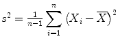 . The SD has the advantage over the variance that it is expressed in the original units of the data. For example, since blood pressure is measured in mmHg, the variance is expressed in mmHg2, while the SD is also expressed in mmHg.
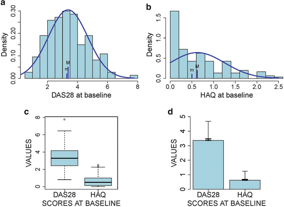
 . This formula shows that when the patient population is homogeneous (small variance) and/or the study is large, there is little variation of the sample mean around the true mean and then taking the study mean for the population mean will not induce a great error. One can also guess the distance between the true and sample mean with the confidence interval (CI). Namely, the 95 % confidence interval given by
 ![$$ \left[\overline{X}-2\times \mathrm{SEM},\overline{X}+2\times \mathrm{SEM}\right] $$](/wp-content/uploads/2016/11/A304262_1_En_2_Chapter_IEq4.gif) contains the true mean with 0.95 probability. Note that the coefficient “2” in the above expression is approximate and varies with the study size, as seen later. Thus, the smaller the 95 % CI, the more precise statement we can make about the true mean. For the RAPPORT study, the SEM of the mean DAS28 at baseline is equal to
contains the true mean with 0.95 probability. Note that the coefficient “2” in the above expression is approximate and varies with the study size, as seen later. Thus, the smaller the 95 % CI, the more precise statement we can make about the true mean. For the RAPPORT study, the SEM of the mean DAS28 at baseline is equal to 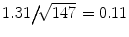 (for some patients, DAS28 is missing), yielding a 95 % CI equal to [3.15, 3.58]. This implies that we are not sure about the true mean of DAS28, but we believe with 95 % certainty that it is greater than 3.15 and smaller than 3.58. For HAQ at baseline, we obtained an
 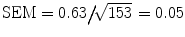 and the 95 % CI now becomes [0.52, 0.72]. Bars have been added in Fig. 1 that represent the SEM.
 and
and  , i.e.,
 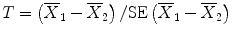 , whereby
  is the standard error of the difference in means (similar to the SEM of a single mean). This standardized difference T is then compared to a reference distribution, here the t–distribution with (n 1 + n 2 − 2) degrees of freedom (df). This distribution reflects the natural variability of T under the null hypothesis that Δ = 0. The degrees of freedom is a parameter that depends on the sample sizes of the groups and determines the particular t-distribution. Note that when df ≥30, the t-distribution becomes close to the normal distribution. For the comparison of the change in DAS28 between men and women, df = 26 + 81 − 2 = 105. Under the null hypothesis one expects that T varies around zero, which translates into a statement that under H 0 there is 95 % chance that T is located between two extreme values roughly equal to −2 and 2 (which change with df). Observed T values outside this central interval thus indicate that the null hypothesis may not be true and correspond to a P-value smaller than 0.05. For the DAS28 comparison, this interval is equal to [−1.983, 1.983]. We obtained T = −0.577, which belongs to the above central interval and therefore P > 0.05. For the comparison of the mean ages between men and women, df = 157 and the central interval is now [−1.975, 1.975]. Since T = −2.836 does not belong to this interval, P < 0.05.
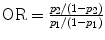 .
. and π B are equal. Suppose the observed proportions under treatments A and B are given by p A and p B, respectively, then the chi-square test computes X 2 = (p A − p B)2/SE(p A − p B)2, with SE(p A − p B) the standard error of the difference in proportions under H 0. When X 2 is too large (compared to what is expected under the null hypothesis), H 0 is rejected (at α = 0.05). For the actual calculation of the P-value, the chi–square distribution with one degree of freedom is used as reference distribution. Table 2 represents a 2 × 2 contingency table contrasting the frequencies of men and women in the RAPPORT study who require step-up treatment (DAS28 > 3.2). This table is a special case of an r × c contingency table when there are r rows and c columns in the table. In Table 2 the lower case symbols stand for the observed frequencies, while the upper case symbols refer to the expected frequencies, i.e., those that one would expect on average to happen under the null hypothesis. Comparing the observed with the expected frequencies leads to an equivalent expression of X 2 given by
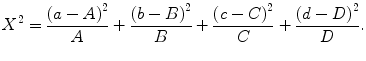
 and the odds ratio
 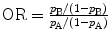 , the value of 1 must not be within the 95 % CI to claim a significant effect. Using the observed frequencies in Table 2, the odds ratio is easily seen to be equal to ad/bc. For the entries in Table 2, we obtained RR = 1.28 with 95 % CI = [0.88, 1.85] and OR = 1.7 with 95 % CI = [0.71, 4.06]. Both intervals do include 1 and hence there is no evidence for a difference in the true proportions between men and women.
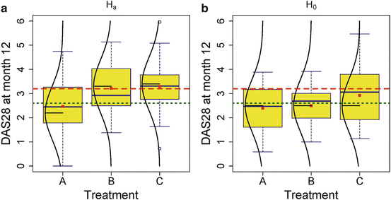
 Medicine in Rheumatology: How Does It Differ from Other Diseases?


