CHAPTER 21 Recent advances in the diagnosis and treatment of glenohumeral bone loss
 An accurate assessment of glenoid bone loss is essential for making an informed surgical decision in patients with glenohumeral instability. The secant method is a novel and accurate technique for measuring glenoid bone loss.


Section I: measuring glenoid bone loss
Accurate quantification of glenoid bone loss in patients with shoulder instability is essential for preoperative planning and informed discussions on the expected outcomes after surgery. The unlikely stability of the uninjured glenohumeral joint is largely attributable to several restraint mechanisms, including the constraining bony articulation and a complex array of dynamic and static mechanisms that work to center the humeral head on the glenoid fossa. The glenoid socket is only 5 mm deep in the anteroposterior (AP) direction,1 so osseous pathology that would otherwise be subtle has a remarkable effect on shoulder instability—a 20% to 25% loss may only be a 6- to 8-mm osseous defect in the anteroinferior glenoid. It is critical to precisely determine the degree of glenoid bone loss in order to select an optimal treatment plan (i.e., arthroscopic/open repair versus bone augmentation procedures) and to fully educate patients on prognosis.
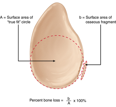
In recent years, new techniques have emerged for preoperative quantification of glenoid bone loss, answering an obvious need for improved accuracy. Baudi et al, in 2005, reported a novel technique called the “Pico method” for quantification using multiplanar reconstruction (MPR) to calculate a percentage defect.2 The Pico method uses a two-dimensional (2-D) computed tomography (CT) view to provide an en face view of the glenoid. A concentric circle is first drawn on the inferior aspect of the contralateral, healthy glenoid and its area (A) is calculated. A circle with identical circumference and radius is then drawn directly onto the inferior portion of the injured glenoid. Bone defect (b) is identified as the missing area of the circle and a percentage is calculated with MPR using the following formula: percent bone loss = b/A × 100%. A similar technique, described by Sugaya et al, relies on three-dimensional (3-D) CT with digital extraction of the humeral head.3 Like the Pico method, a best fit true circle is drawn on the inferior portion of a pear-shaped glenoid contour on an en face view. Surface areas of the best fit circle and the osseous defect are digitally measured. Glenoid bone loss is subsequently computed by dividing the surface area of the bony defect by the total surface area of the circle (Fig. 21-1). Osseous defects are graded as medium sized if they represent 5% to 20% of the glenoid fossa; anything above or below this range is classified as either large or small.
In addition to using CT for preoperative bone loss measurements, osseous defects in the glenoid also can be measured during arthroscopy using a 3- to 4-mm calibrated probe. Central to the methods for arthroscopic quantification is the concept that the inferior glenoid is circularly shaped.4,5 Simple geometry can then be employed to calculate percent bone loss by computing surface areas, much like the radiographic methods previously described. Even though there is little controversy regarding the circular morphology of the inferior glenoid, the true center point (focus) of this circle is often debated.
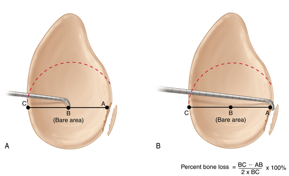
The glenoid bare spot (GBS), a thinning in cartilaginous covering and increased subchondral density that overlies the tubercle of Assaki, has been frequently reported to be a functional center point for the inferior glenoid circle. Using measurements taken from both fresh frozen cadavers and live subjects undergoing arthroscopy, Burkhart et al showed the GBS to be consistently equidistant from the anterior, posterior, and inferior glenoid margins.4 The authors then described a unique technique, the GBS method, for computing percentage bone loss. To perform the GBS method, first insert a 3- to 4-mm calibrated probe into the posterior portal of the shoulder (while viewing through the anterosuperior portal) and measure the distance from the GBS to the posterior glenoid rim at the level of the bare spot (BC) (Fig. 21-2, A). Advance the probe such that the tip is flush with the anterior edge of the osseous defect (Fig. 21-2, B); this distance from the bare area to the anterior edge should be recorded (AB). In order to calculate percent bone loss, the following formula can be used: percent bone loss = (BC − AB)/2BC × 100%.4,6
Although the GBS method is a popular and straightforward way to quantify osseous defects, its validity in certain cases recently has been questioned. In 2008, Provencher et al used cadaveric shoulders to compare the accuracy of the GBS method when osseous defects were 45 degrees and 0 degrees relative to the long axis of the glenoid.7 Using osteotomies to simulate bony Bankart defects, the authors concluded that the GBS method is accurate when bone loss occurs parallel to the long axis of the glenoid. If the osseous defect lies at a 45-degree angle relative to the long axis, arthroscopic measurement from either the 2-o’clock or 3-o’clock posterior portal will significantly overestimate the amount of true bone loss. Other authors also have shown problems with using the GBS method, many of whom have questioned the assumption that the glenoid bare spot is the true center point of the inferior glenoid circle. In a recent anatomic study examining the location of the glenoid bare spot with respect to the focus of the inferior glenoid circle, Kralinger et al used CT verification to demonstrate that the glenoid bare spot is approximately 1.4 mm anterior to the true center point.8 If the anatomic landmark denoting the center point of the inferior glenoid circle is situated too anteriorly, the GBS method may once again consistently overestimate the amount of true bone loss.
A recently proposed technique for glenoid bone loss quantification aims to avoid problems associated with the GBS by relying on the secant cord theorem (SCT).9 In simple terms, a secant is a straight line that intersects the circumference of a circle twice and extends beyond the radius (Fig. 21-3, A). When two secants share an endpoint outside of a circle, the products of their lengths and external segments are equal. In other words, DE × ME = FE × NE according to Figure 21-3, A. By solving for FN, one can derive the formula: FN = (DE × ME/NE) − NE.9
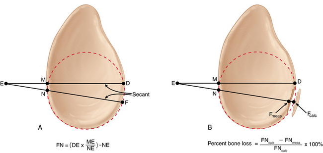
In order to quantify glenoid osseous defects using the SCT method, use a 3 to 4 mm calibrated probe to measure the segments DE, ME, and NE as shown in Figure 21-3. Next, calculate the theoretic value of FN (FNcalc) using the formula FNcalc = (DE × ME/NE) − NE. The actual value of FN (FNmeas) is then measured intra-articularly using the calibrated probe. Percent bone loss is determined as follows: percent bone loss = (FNcalc − FNmeas)/ FNcalc × 100% (Fig. 21-3, B).
An accurate assessment of glenoid bone loss is essential for making an informed surgical decision in patients with glenohumeral instability. Even a 10% to 15% error in quantification may have profound effects on surgical decision making by misleading the orthopaedic surgeon into pursuing an ineffective surgical solution. As demonstrated in the literature, CT examination and arthros- copy have a high degree of correlation with respect to the degree of bone loss.10,11 By verifying findings using both radiographic and arthroscopic techniques, a more complete picture of glenoid bone loss may be achieved.
Section II—bipolar glenoid and humeral bone defects
Introduction
Traditionally, each has been studied in isolation as a risk factor for recurrent instability. However, the most recent literature suggests that humeral and glenoid bone deficiencies are intimately related to each other.12 It is best viewed as a bipolar problem that can be a key contributor to recurrent instability events. Therefore, bone loss on both sides of the joint must be considered and often addressed in concert to afford the patient the best possible outcome.
Epidemiology
There is wide variability in the reported rates of humeral and glenoid bone defects, which is most likely due to a lack of uniformity in methods of identifying these injuries. The incidence of Hill-Sachs lesions in anterior shoulder instability ranges from 38% to 88% and is associated with up to 100% of recurrent dislocations.13 The reported rate of glenoid bone deficiency in first-time dislocators is approximately 20%, and it is up to 90% in patients with recurrent instability.14,15
Pathophysiology
The Hill-Sachs lesion is classically described as a compression fracture of the posterosuperolateral humeral head in association with anterior instability or dislocation of the glenohumeral joint. It was radiographically described by Hill and Sachs as a line of condensation on the internal rotation shoulder radiograph and was attributed to the impression of the dense cortical glenoid on the humeral head during an anterior dislocation event. The location and orientation of the lesion is based solely on the position of the humeral head when it comes into contact with the anterior glenoid. This is not necessarily the position of the shoulder at the time of dislocation.16
In contrast to humeral-sided lesions, glenoid osseous injuries are more variable in morphology with a wider range of proposed mechanisms. However, the location of these lesions is well defined and almost always occurs in the anterior inferior quadrant of the glenoid. Saito et al found that most injuries occurred between 2:30 and 4:20 when the glenoid was depicted as a clock face.17
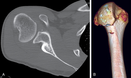
Though the exact mechanism of glenoid injury is unknown it can be theorized based on the radiographic and arthroscopic characteristics of the lesion. Large fractures may be due to an axial load on the anteroinferior glenoid, whereas smaller lesions are probably due to an avulsion mechanism. Most of these avulsion fractures are small or medium in size.3 In other cases, no true fracture of the glenoid is identified, but the bone is abnormal with “erosive” changes. Sugaya et al evaluated the glenoid with 3-D CT and noted this finding in 40% of patients with recurrent anterior instability.3 This blunted lesion may be caused by acute marginal impaction of the glenoid, or it may be due to a chronic, erosive mechanism secondary to recurrent instability (Fig. 21-4).
Related posts:
 Open surgical solutions for posterior instability of the shoulder
 Clinical history, examination, arthroscopic findings, and treatment of multidirectional instability
 Recognition and management of combined instability and rotator cuff tears
 Open treatment of multidirectional instability—surgical technique
 Humeral head defects—biomechanics, measurements, and treatments
 Nonoperative rehabilitation for traumatic and atraumatic glenohumeral instability
Stay updated, free articles. Join our Telegram channel

Full access? Get Clinical Tree


