2 Normal gait
Walking and gait
As walking is such a familiar activity, it is difficult to define it without sounding pompous. However, it would be remiss not to attempt a definition. Normal human walking and running can be defined as ‘a method of locomotion involving the use of the two legs, alternately, to provide both support and propulsion’. In order to exclude running, we must add ‘at least one foot being in contact with the ground at all times’. Unfortunately, this definition excludes some forms of pathological gait which are generally regarded as being forms of walking, such as the ‘three-point step-through gait’ (see Fig. 3.21), in which there is an alternate use of two crutches and either one or two legs. It is probably both unreasonable and pointless to attempt a definition of walking which will apply to all cases – at least in a single sentence!
History
The history of gait analysis has shown a steady progression from early descriptive studies, through increasingly sophisticated methods of measurement, to mathematical analysis and mathematical modelling. Only a brief account of the development of the discipline will be given here. Good reviews of the early years of gait analysis have been given by Garrison (1929), Bresler and Frankel (1950) and Steindler (1953). The more recent history of gait analysis, and of clinical gait analysis in particular, was covered in three excellent review papers by Sutherland (2001, 2002, 2005).
Muscle activity
For a full understanding of normal gait, it is necessary to know which muscles are active during the different parts of the gait cycle. The role of the muscles was studied by Scherb, in Switzerland, during the 1940s, initially by palpating the muscles as his subject walked on a treadmill, then later by the use of electromyography (EMG). Further advances in the understanding of muscle activity and many other aspects of normal gait were made during the 1940s and 1950s by a very active group working in the University of California at San Francisco and Berkeley, notable among whom was Verne Inman. This group later went on to write Human Walking (Inman et al., 1981), published just after Inman’s death, which to many people is the definitive textbook on normal gait. This has now gone through several editions, the latest edition of this being Rose and Gamble (2005). Another classic text on EMG is Muscles Alive: Their Functions Revealed by Electromyography by John Basmajian, which unfortunately has not been updated since 1985.
The use of EMG in gait analysis has received much attention but perhaps the most influential paper published was ‘The use of surface electromyography in biomechanics’ by Carlo De Luca in 1997, which gave a summary of recommendations but perhaps more importantly a summary of problems which at the time needed resolution. Further standardisation was achieved through the SENIAM (Surface ElectroMyoGraphy for the Non-Invasive Assessment of Muscles) project coordinated and managed by Hermie Hermens and Bart Freriks from Enschede, which is now considered by many as the definitive recommendations for electrode configuration and sensor positioning on specific muscles.
Mechanical analysis
A major contribution to the mechanical analysis of walking, also from the Californian group, was made by Bresler and Frankel (1950). They performed free-body calculations for the hip, knee and ankle joints, allowing for ground reaction forces, the effects of gravity on the limb segments and the inertial forces. The analytical techniques developed by these workers formed the basis of many current methods of modelling and analysis.
An important paper describing the possible mechanisms which the body uses to minimise energy consumption in walking, again from California, was published by Saunders et al. (1953). Further important work on energy consumption and in particular the energy transfers between the body segments in walking, was published by Cavagna and Margaria (1966), working in Italy. By 1960, research began to concentrate on the variability of walking, the development of gait in children and the deterioration of gait in old age. Patricia Murray, working in Milwaukee, Wisconsin, published a series of papers on these subjects, including a detailed review (Murray, 1967).
Mathematical modelling
Once the motions of the body segments and the actions of the different muscles had been examined and documented, attention passed to the forces generated across the joints. Although limited calculations of this type had been made previously, the study by Paul (1965) was the first detailed analysis of hip joint forces during walking. A subsequent paper by the same author also included an analysis of the forces in the knee (Paul, 1966). Since then there have been many mathematical studies of force generation and transmission across the hip, knee and ankle.
Clinical application
As well as a gradual increase in the clinical use of scientific gait analysis, there has also been a growing interest in the use of observational or visual gait analysis. This has become much easier to perform since digital video cameras have become widely available, which is reviewed in more detail by Sutherland (2001, 2002, 2005).
Terminology used in gait analysis
The gait cycle is defined as the time interval between two successive occurrences of one of the repetitive events of walking. Although any event could be chosen to define the gait cycle, it is generally convenient to use the instant at which one foot contacts the ground (‘initial contact’). If it is decided to start with initial contact of the right foot, as shown in Figure 2.1, then the cycle will continue until the right foot contacts the ground again. The left foot, of course, goes through exactly the same series of events as the right, but displaced in time by half a cycle.
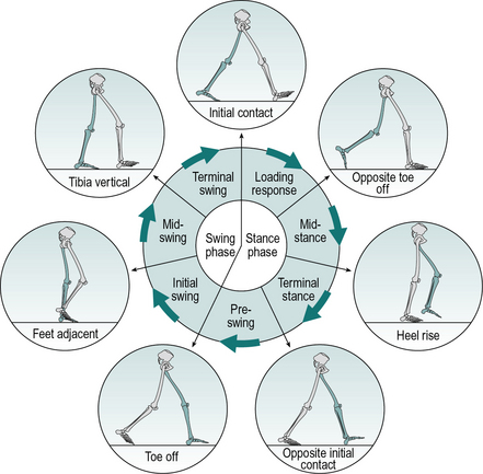
The following terms are used to identify major events during the gait cycle:
These seven events subdivide the gait cycle into seven periods, four of which occur in the stance phase, when the foot is on the ground, and three in the swing phase, when the foot is moving forward through the air (Fig. 2.1). The stance phase, which is also called the ‘support phase’ or ‘contact phase’, lasts from initial contact to toe off. It is subdivided into:
The swing phase lasts from toe off to the next initial contact. It is subdivided into:
The duration of a complete gait cycle is known as the cycle time, which is divided into stance time and swing time. Unfortunately, the nomenclature used to describe the gait cycle varies considerably from one publication to another. The present text attempts to use terms which will be understood by most people working in the field; alternative terminology will be given where appropriate. Wall et al. (1987) pointed out that the usual terminology is inadequate to describe some severely pathological gaits.
Gait cycle timing
Figure 2.2 shows the timings of initial contact and toe off for both feet during a little more than one gait cycle. Right initial contact occurs while the left foot is still on the ground and there is a period of double support (also known as ‘double limb stance’) between initial contact on the right and toe off on the left. During the swing phase on the left side, only the right foot is on the ground, giving a period of right single support (or ‘single limb stance’), which ends with initial contact by the left foot. There is then another period of double support, until toe off on the right side. Left single support corresponds to the right swing phase and the cycle ends with the next initial contact on the right.
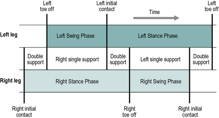
In each gait cycle, there are thus two periods of double support and two periods of single support. The stance phase usually lasts about 60% of the cycle, the swing phase about 40% and each period of double support about 10%. However, this varies with the speed of walking, the swing phase becoming proportionately longer and the stance phase and double support phases shorter, as the speed increases (Murray, 1967). The final disappearance of the double support phase marks the transition from walking to running. Between successive steps in running there is a flight phase, also known as the ‘float’, ‘double-float’ or ‘non-support’ phase, when neither foot is on the ground. A detailed study of gait cycle timing was published by Blanc et al. (1999).
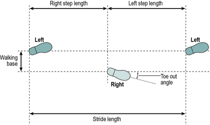
Foot placement
The terms used to describe the placement of the feet on the ground are shown in Figure 2.3. The stride length is the distance between two successive placements of the same foot. It consists of two step lengths, left and right, each of which is the distance by which the named foot moves forward in front of the other one. In pathological gait, it is common for the two step lengths to be different. If the left foot is moved forward to take a step and the right one is brought up beside it, rather than in front of it, the right step length will be zero. It is even possible for the step length on one side to be negative, for example, if the left foot never catches up with the right foot, the distance between the left and right feet will be negative. However, the stride length starting with the left heel strike must always be the same as the stride length starting with the right heelstrike, unless the subject is walking around a curve where the inside leg will have a shorter stride length than the outside leg. This definition of a ‘stride’, consisting of one ‘step’ by each foot, breaks down in some pathological gaits, in which one foot makes a series of ‘hopping’ movements while the other is in the air (Wall et al., 1987). There is no satisfactory nomenclature to deal with this situation.
It is common experience that you need to walk more carefully on ice than on asphalt. Whether or not the foot slips during walking depends on two things: the coefficient of friction between the foot and the ground, and the relationship between the vertical force and the forces parallel to the walking surface (front-to-back and side-to-side). The ratio of the horizontal to the vertical force is known as the ‘utilised coefficient of friction’ and slippage will occur if this exceeds the actual coefficient of friction between the foot and the ground. In normal walking, a coefficient of friction of 0.35–0.40 is generally sufficient to prevent slippage; the most hazardous part of the gait cycle for slippage is initial contact. There is a fairly extensive literature on foot-to-ground friction and slippage, e.g. Cham and Redfern (2002) and Burnfield et al. (2005).
Cadence, cycle time and speed
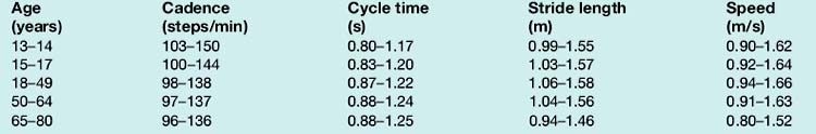
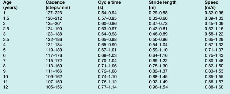
The cadence is the number of steps taken in a given time, the usual unit being steps per minute. In most other types of scientific measurement, complete cycles are counted, but as there are two steps in a single gait cycle, the cadence is a measure of half-cycles. The normal ranges for both cadence and cycle time in both sexes at different ages are showed in Table 1 at the end of this chapter, where we consider the effect of age in more detail.
Table 1 Normal ranges for gait parameters
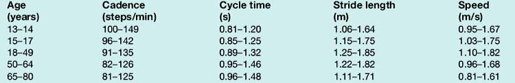
Approximate range (95% limits) for general gait parameters in free-speed walking by normal CHILDREN of different ages (ages 1–7 years based on Sutherland et al. (1988))

If cycle time is used in place of cadence, the calculation becomes much more straightforward:

When making comparisons between individuals, particularly with children, it is useful to allow for differences in size. This is done by dividing a measurement by some aspect of body size, such as height (stature) or leg length, a procedure generally known as ‘normalisation’. It is thus fairly common to see walking speed expressed in ‘statures per second’ or to see measures such as ‘step factor’, which is step length divided by leg length (Sutherland, 1997).
Since walking speed depends on both cadence and stride length, it follows that speed may be changed by altering only one of these variables, for instance by increasing the cadence while keeping the stride length constant. In practice, however, people normally change their walking speed by adjusting both cadence and stride length. Sekiya and Nagasaki (1998) defined the ‘walk ratio’ as step length (m) divided by step rate (steps/min) and found that it was fairly constant in both males and females over a range of walking speeds from very slow to very fast. Macellari et al. (1999) made a detailed study of the relationships between gender, body size, walking speed, gait timing and foot placement.
Outline of the gait cycle
The purpose of this section is to provide the reader with an overview of the gait cycle, to make the detailed description which follows a little easier to follow. The cycle is illustrated by Figures 2.4 and 2.10–2.18, all of which are taken from a single walk by a 22-year-old normal female, weight 540 N (55 kg, 121 lb), walking barefoot with a cycle time of 0.88 s (cadence 136 steps/min), a stride length of 1.50 m and a speed of 1.70 m/s. The individual measurements from this subject do not always correspond to ‘average’ values, because of the normal variability between individuals, although they are all close to the normal range. The measurements were all made in the plane of progression, which is a vertical plane aligned to the direction of the walk; in normal walking it closely corresponds to the sagittal plane of the body. The data were obtained using a Vicon motion system and a Bertec force platform. It should be noted that different laboratories use different methods of measurement, so that other publications may quote different values for some of the measured variables. The reader should thus concentrate on the changes in the variables during the gait cycle, rather than on their absolute values.
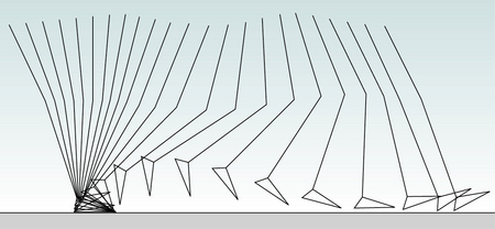
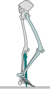
Fig. 2.4 • Position of the right leg in the sagittal plane at 40 ms intervals during a single gait cycle.
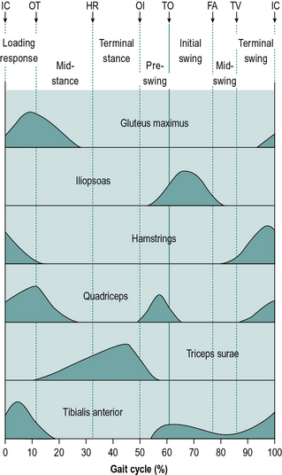
Fig. 2.10 • Typical activity of major muscle groups during the gait cycle. Abbreviations as in Figure 2.5. The timings of the events of the gait cycle are typical and not derived from a single subject.
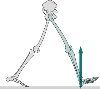
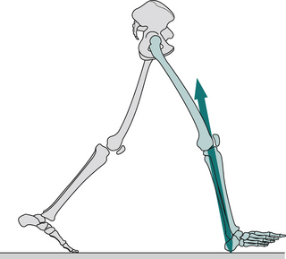
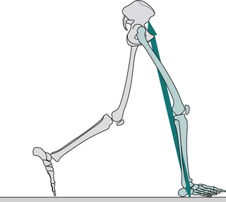
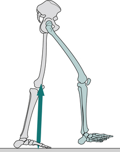
Fig. 2.13 • Opposite toe off: position of right leg (green), left leg (grey) and ground reaction force vector.
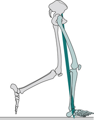
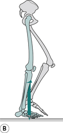
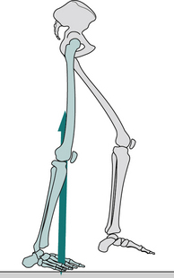
Fig. 2.15 • Heel rise: position of right leg (green), left leg (grey) and ground reaction force vector.
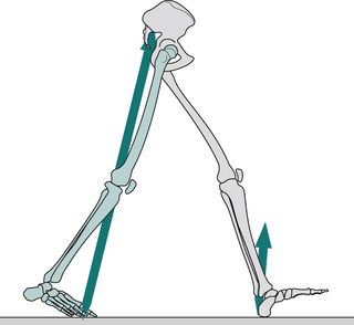
Fig. 2.16 • Opposite initial contact: position of right leg (green), left leg (grey) and ground reaction force vector.
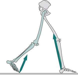
Fig. 2.17 • Toe off: position of right leg (green), left leg (grey) and ground reaction force vector.
The descriptions which follow assume that symmetry is present between the two sides of the body. This is approximately true for normal individuals, although detailed examination shows that everyone has some degree of asymmetry (Sadeghi, 2003). Such subtle asymmetries are negligible, however, when contrasted with the majority of pathological gaits.
Some gait studies are performed barefoot and some with the subject wearing shoes. Oeffinger et al. (1999) found small differences in some of the gait parameters between these two conditions in children, but did not consider them to be clinically significant. It is usually at the discretion of the investigator whether or not shoes are worn, although in some cases (e.g. when an ankle–foot orthosis or an orthotic insole is used) this may be dictated by the subject’s condition.
During gait, important movements occur in all three planes – sagittal, frontal and transverse. However, this introductory text will concentrate on the sagittal plane, in which the largest movements occur. For information on the motion in other planes, the reader is referred to more detailed texts, such as Perry (1992), Inman et al. (1981) or Rose and Gamble (1994). Figure 2.4 shows the successive positions of the right leg at 40 ms intervals, measured over a single gait cycle. Figure 2.5 shows the corresponding sagittal plane angles at the hip, knee and ankle joints and Figure 2.6 shows the sagittal plane angular velocity of the hip, knee and ankle joints.
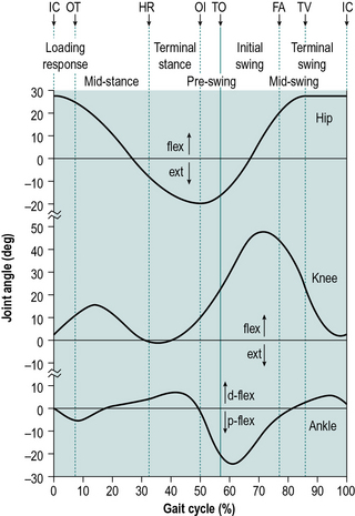
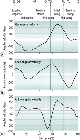
Figure 2.7 shows the internal joint moments (in newton-metres per kilogram body mass) and Figure 2.8 the joint powers (in watts per kilogram body mass). Different authors have used different units for the measurement of moments and powers; those used here are scaled for body mass, but not for the length of the limb segments. In Figure 2.8, the annotations H1–H3, K1–K4 and A1–A2 refer to the peaks of power absorption and generation described by Winter (1991).
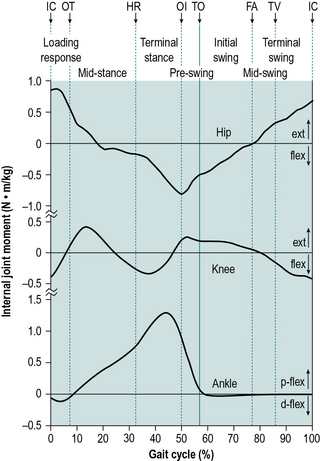
Fig. 2.7 • Sagittal plane internal joint moments (newton-metres per kilogram body mass) during a single gait cycle of right hip (extensor moment positive), knee (extensor moment positive) and ankle (plantarflexor moment positive). Abbreviations as in Figure 2.5.
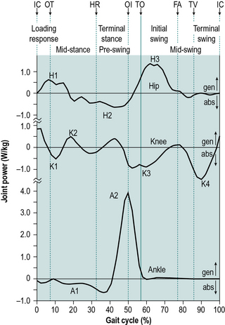
Fig. 2.8 • Sagittal plane joint powers (watts per kilogram body mass) during a single gait cycle of right hip, knee and ankle. Power generation is positive, absorption is negative. See text for meaning of H1, H2, etc. Other abbreviations as in Figure 2.5.
Figure 2.9 shows a ‘butterfly diagram’, described by Pedotti (1977). This is a plot of the ground reaction vectors and is made up of successive representations, at 10 ms intervals, of the magnitude, direction and point of application of the ground reaction force vector. The vectors move across the diagram from left to right and create a shape that resembles the wings of a butterfly.
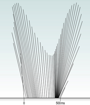
Figure 2.10 gives the typical activity of a number of key muscles or muscle groups during the gait cycle. It is based largely on data from Perry (1992), Inman et al. (1981) and Rose and Gamble (1994). Similar, though not identical, data for these and other muscles were given by Sutherland (1984) and Winter (1991). Although Figure 2.10 shows a typical pattern, it is not the only possible one. One of the interesting things about gait is the way in which the same movement may be achieved in a number of different ways and this particularly applies to the use of muscles, so that two people may walk with the same ‘normal’ gait pattern but using different combinations of muscles. The pattern of muscle usage not only varies from one subject to another but it is also affected by fatigue and varies with walking speed, in a single person. The muscular system is said to possess ‘redundancy’, which means that if a particular muscle cannot be used, its functions may be taken over another muscle or group of muscles. A good review of muscle activity in gait was provided by Shiavi (1985).
Figures 2.11–2.19 show the positions of the two legs and the ground reaction force vector beneath the right foot (where present), at the seven major events of the gait cycle and at two additional points – near the beginning of the loading response (Fig. 2.12) and halfway through mid-stance (Fig. 2.14). The description is based on a gait cycle from right initial contact to the next right initial contact. However, the gait cycle could just as easily have been defined using the left leg.
Throughout the text, references will be made to the position of the ground reaction force vector relative to the axis of a joint and to the resulting joint moments. This approach, known as ‘vector projection’, is an approximation at best, since it neglects the mass of the leg below the joint in question (especially important at the hip) and also ignores the acceleration and deceleration of the limb segments (which primarily lead to errors in the swing phase). However, the author has used this approach since it makes it much easier to understand joint moments. The graphs for joint moments (Fig. 2.7) and joint powers (Fig. 2.8) were calculated ‘correctly’, using a method known as ‘inverse dynamics’, which is based on the kinematics, the ground reaction force and the subject’s anthropometry. Wells (1981) discussed the relative merits of these two methods for estimating joint moments.
Upper body
The upper body moves forwards throughout the gait cycle. Its speed varies a little, being fastest during the double support phases and slowest in the middle of the stance and swing phases. The trunk twists about a vertical axis, the shoulder girdle rotating in the opposite direction to the pelvis. The arms swing out of phase with the legs, so that the left leg and the left side of the pelvis move forwards at the same time as the right arm and the right side of the shoulder girdle. Lamoth et al. (2002) made a detailed study of the relative motion between the pelvis and the trunk at different walking speeds. Murray (1967) found average total excursions of 7° for the shoulder girdle and 12° for the pelvis, in adult males walking at free speed. The fluidity and efficiency of walking depend to some extent on the motions of the trunk and arms, but these movements are commonly ignored in clinical gait analysis and have been relatively neglected in gait research. The whole trunk rises and falls twice during the cycle, through a total range of about 46 mm (Perry, 1992), being lowest during double support and highest in the middle of the stance and swing phases. An approximation to this vertical motion can be seen in the position of the hip joint in Figure 2.4. The trunk also moves from side to side, once in each cycle, the trunk being over each leg during its stance phase, as might be expected from the need for support. The total range of side-to-side movement is also about 46 mm (Perry, 1992). The pelvis, as well as twisting about a vertical axis, also tips slightly, both backwards and forwards (with an associated change in lumbar lordosis) and from side to side. The spinal muscles are selectively activated so that the head moves less than the pelvis, which is important for providing a stable platform for vision (Prince et al., 1994).
Hip
The hip flexes and extends once during the cycle (Fig. 2.5). The limit of flexion is reached around the middle of the swing phase and the hip is then kept flexed until initial contact. The peak extension is reached before the end of the stance phase, after which the hip begins to flex again.
The gait cycle in detail
More detailed descriptions of the events of normal gait are given by Murray (1967), Perry (1992), Inman et al. (1981) and Rose and Gamble (1994).
Initial contact (Fig. 2.11)
1 General:
Initial contact is the beginning of the loading response, which is the first period of the stance phase. Initial contact is frequently called ‘heelstrike’, since in normal individuals there is often a distinct impact between the heel and the ground, known as the ‘heelstrike transient’. Other names for this event are ‘heel contact’, ‘footstrike’ or ‘foot contact’. The direction of the ground reaction force changes from generally upwards during the heelstrike transient (Fig. 2.11) to upwards and backwards in the loading response, immediately afterwards (Fig. 2.12). This change in direction can also be seen in the butterfly diagram (Fig. 2.9), where the force vector changes direction immediately after initial contact.
2 Upper body:
The trunk is about half a stride length behind the leading (right) foot at the time of initial contact. In the side-to-side direction, the trunk is crossing the midline in its range of travel, moving towards the right, as the foot on that side makes contact. The trunk is twisted, the left shoulder and the right side of the pelvis each being at their furthest forwards and the left arm at its most advanced. The amount of arm swinging varies greatly from one person to another and it also increases with the speed of walking. At the time of initial contact, Murray (1967) found the mean elbow flexion was 8° and the shoulder flexion 45°.
3 Hip:
The attitude of the legs at the time of initial contact is shown in Fig. 2.11. The maximum flexion of the hip (generally around 30°) is reached around the middle of the swing phase, after which it changes little until initial contact. The hamstrings are active during the latter part of the swing phase (since they act to prevent knee hyperextension); gluteus maximus begins to contract around the time of initial contact and together these muscles start the extension of the hip, which will be complete around the time of opposite initial contact (Fig. 2.5).
4 Knee:
The knee extends rapidly at the end of the swing phase, becoming more or less straight just before initial contact and then starting to flex again (Figs 2.5 and 2.11). This extension is generally thought to be passive, although Perry (1992) states that it involves quadriceps contraction. Except in very slow walking, the hamstrings contract eccentrically at the end of the swing phase, to act as a braking mechanism to prevent knee hyperextension. This contraction continues into the beginning of the stance phase.


Stay updated, free articles. Join our Telegram channel

Full access? Get Clinical Tree


