Chapter 3 Materials science
Despite publicity for exotic materials, no single material is a panacea. One reason is that a single design frequently requires divergent mechanical properties (e.g., stiffness and flexibility required in an ankle–foot orthosis [AFO] for dorsiflexion restraint and free plantar flexion). In addition, practitioners rarely are presented with situations where they will use only one material or with single-design situations that will not require modification, customization, or variation over time.
Strength and stress
 (3-1)
(3-1)Where F = applied force (pounds or Newtons), and A = cross-sectional area (square inches or square meters).
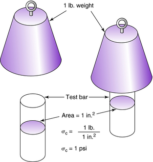
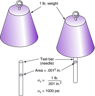
The same amount of force applied over different areas causes radically different stresses. For example, a 1-lb weight is placed on a cylindrical test bar having a cross-sectional area of 1 in2. According to Equation 3-1, the compressive stress σc in the cylindrical test bar is 1 lb/in2 (Fig. 3-1). When the same 1-lb weight is placed on a needle having a cross-sectional area of 0.001 in2, the compressive stress σc in the needle is 1000 psi (Fig. 3-2).
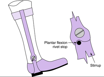
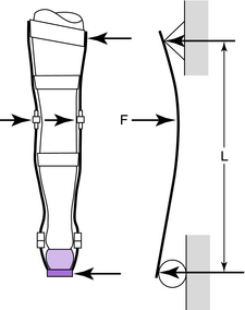
Similar problems are encountered in orthoses and prostheses. A child weighing 100 lb and wearing a weight-bearing orthosis with a 90-degree posterior stop (Fig. 3-3) can exert forces at initial contact that create stresses of thousands of pounds per square inch. If the child jumps, the force would increase with the height of the jump. The stress at the stop or on the rivet could be great enough to cause failure.
Tensile, compressive, shear, and flexural stresses
Materials are subject to several types of stresses depending on the way that the forces are applied: tensile, compressive, shear, and flexural.
Tensile stresses
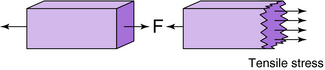
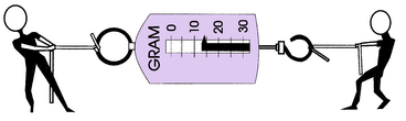
Tensile stresses act to pull apart an object or cause it to be in tension. Tensile stresses occur parallel to the line of force but perpendicular to the area in question (Fig. 3-4). If an object is pulled at both ends, it is in tension, and sufficient force will pull it apart. Two children fighting over a fish scale and exerting opposing forces put it in tension, as shown by the indicator on the scale (Fig. 3-5).
Compressive stresses
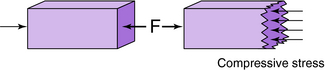
Compressive stresses act to squeeze or compress objects. They also occur parallel to the line of force and perpendicular to the cross-sectional area (Fig. 3-6).
Shear stresses
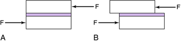
Shear stresses act to scissor or shear the object, causing the planes of the material to slide over each other. Shear stresses occur parallel to the applied forces. Consider two blocks (Fig. 3-7, A) with their surfaces bonded together. If forces acting in opposite directions are applied to these blocks, they tend to slide over each other. If these forces are great enough, the bond between the blocks will break (Fig. 3-7, B). If the area of the bonded surfaces were increased, however, the effect of the forces would be distributed over a greater area. The average stress would be decreased, and there would be increased resistance to shear stress.
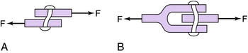
A common lap joint and clevis joint are examples of a shear pin used as the axis of the joint (Fig. 3-8). The lap joint has one shear area of the rivet resisting the forces applied to the lap joint (Fig. 3-8, A), and the rivet in the box joint (clevis) has an area resisting the applied forces that is twice as great as the area in the lap joint (assuming that the rivets in both joints are the same size; Fig. 3-8, B). Consequently the clevis joint will withstand twice as much shear force as the lap joint. The lap joint also has less resistance to fatigue (fluctuating stress of relatively low magnitude, which results in failure) because it is more susceptible to flexing stresses.
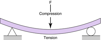
Flexural stress
Flexural stress (bending) is a combination of tension and compression stresses. Beams are subject to flexural stresses. When a beam is loaded transversely, it will sag. The top fibers of a beam are in maximum compression while the bottom side is in maximum tension (Fig. 3-9). The term fiber, as used here, means the geometric lines that compose the prismatic beam. The exact nature of these compressive and tensile stresses are discussed later.
Strain
 (3-2)
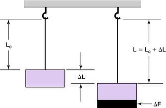
(3-2)Consider a change in length ΔL of a wire or rod caused by a change in stretching force F (Fig. 3-10). The amount of stretch is proportional to the original length of wire. A wire 5 inches long stretches twice as much as a wire 3 to 5 inches long, other things being equal.
Stress–strain curve
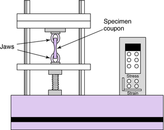
The most widely used means of determining the mechanical properties of materials is the tension test. Much can be learned from observing the data collected from such a test. In the tension test, the dimensions of the specimen coupon are fixed by standardization so that the results can be universally understood, no matter where or by whom the test is conducted. The specimen coupon is mounted between the jaws of a tensile testing machine, which is simply a device for stretching the specimen at a controlled rate. As defined by standards, the cross-sectional area of the coupon is smaller in the center to prevent failures where the coupon is gripped. The specimen’s resistance to being stretched and the linear deformations are measured by sensitive instrumentation (Fig. 3-11).
The force of resistance divided by the cross-sectional area of the specimen is the stress in the specimen (Equation 3-1). The strain is the total deformation divided by the original length (Equation 3-2). If the stresses in the specimen are plotted as ordinates of a graph, with the accompanying strains as abscissae, a number of mechanical properties are graphically revealed. Figure 3-12 shows such a stress–strain diagram for a mild steel specimen.
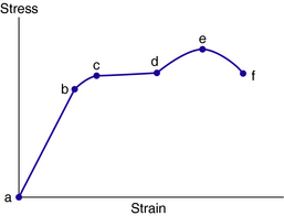
The general shape of the stress–strain curve (Fig. 3-12) requires further explanation. In the region from a to b, the stress is linearly proportional to strain and the strain is elastic (i.e., the stressed part returns to its original shape when the load is removed). When the applied stress exceeds the yield strength, b the specimen undergoes plastic deformation. If the load is subsequently reduced to zero, the part remains permanently deformed. The stress required to produce continued plastic deformation increases with increasing plastic strain (points c, d, and e on Fig. 3-12), that is, the metal strain hardens. The volume of the part remains constant during plastic deformation, and as the part elongates, its cross-sectional area decreases uniformly along its length until point e is reached. The ordinate of point e is the tensile strength of the material. After point e, further elongation requires less applied stress until the part ruptures at point f (breaking or fracture strength). Although this seems counterintuitive, it actually occurs and is best sensed when bolts are overtorqued. Correct torque settings should always be complied with, but practitioners commonly torque bolts using the “as hard as possible” technique, assuming that this method somehow secures the bolt more appropriately than the correct torque and a thread locking solution. When excessive torque has been applied, the bolt first feels like it has loosened prior to failing. This simply reflects the fact that the yield point of the material has been surpassed and the bolt is plastically deforming under a decreasing load to failure.
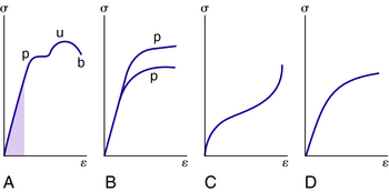
Stress–strain diagrams assume widely differing forms for various materials. Figure 3-13, A shows the stress–strain diagram for a medium-carbon structural steel. The ordinates of points p, u, and b are the yield point, tensile strength, and breaking strength, respectively. The lower curve of Fig. 3-13, B is for an alloy steel and the higher curve is for hard steels. Nonferrous alloys and cast iron have the form shown in Fig. 3-13, C. The plot shown in Fig. 3-13, D is typical for rubber.
For any material having a stress–strain curve of the form shown in Figs. 3-13, A–D, it is evident that the relation between stress and strain is linear for comparatively small values of the strain. This linear relationship between elongation and the axial force causing it was first reported by Sir Robert Hooke in 1678 and is called Hooke’s law. Expressed as an equation, Hooke‘s law becomes:
 (3-3)
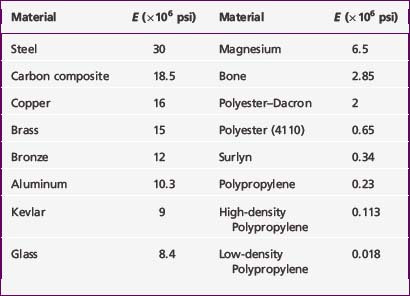
(3-3)The slope of the stress–strain curve from the origin to point p (Figs. 3-13, A and B) is the modulus of elasticity of that particular material E. The region where the slope is a straight line is called the elastic region, where the material behaves in what we typically associate as an elastic manner, that is, it is loaded and stretched, and upon releasing the load the material returns to its original position. The ordinate of a point coincident with p is known as the elastic limit (i.e., the maximum stress that may develop during a simple tension test such that no permanent or residual deformation occurs when the load is entirely removed). Values for E are given in Table 3-1.
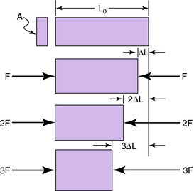
In a routine tension test (Fig. 3-14), which illustrates Hooke’s law, a bar of area A is placed between two jaws of a vise, and a force F is applied to compress the bar. Combining Equations 3-1, 3-2, and 3-3 and solving for the shortening ΔL gives:
 (3-4)
(3-4)Because the original length L0, cross-sectional area A, and modulus of elasticity E are constants, the shortening ΔL depends solely on F. As F doubles, so does ΔL.
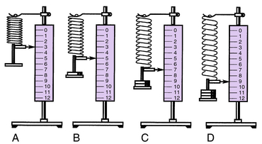
The operation of a steel spring scale is another practical illustration of Hooke’s law (Fig. 3-15). The amount of deflection of the spring for every pound of force of the load remains constant. In Fig. 3-15, A, the scale indicates three units (pounds, ounces, grams). With one weight added (Fig. 3-15, B), the scale indicates 5, or two additional units. A second weight added (Fig. 3-15, C) causes the scale to indicate 7, or a total of four additional units, and a third weight stretches the spring two more units (Fig. 3-15, D). Therefore, it is possible to make uniform gradations for every unit of force to the point beyond the range of elasticity where the spring would distort or break. Scales are manufactured with springs strong enough to bear predetermined maximum loads. A compression spring scale designed to remain within the elastic range, recording weights to about 250 lb (100 kg) and then returning back to 0, is the common type used for weighing people.
Plastic range
Plastic range is beyond the elastic range (b to past e on the stress–strain diagram of Fig. 3-12), and the material behaves plastically. That is, the material has a set or permanent deformation when externally applied loads are removed—it has “flowed” or become plastic. In the case of the steel spring scale, if the weight did not actually break the spring, it would stretch it permanently so that the readings on the scale would be no longer accurate.
When forming orthotic bars, the practitioner must bend the bar beyond the elastic limit and into a range of plastic deformation with some associated elastic return. With experience and some basic experiments, the practitioner will be able to accurately predict the range of deformation and return for particular bends. An advisable strategy is to chart this elastic return for the regular bends and commonly used sidebars.
For most materials, the stress–strain curve has an initial linear elastic region in which deformation is reversible. Note the load σ2 in Fig. 3-16. This load will cause strain εE. When the load is removed, the strain disappears, that is, point X (σ2, εE) moves linearly down the proportional portion of the curve to the origin. Similarly, when load σ1 is applied, strain εT results. However, when load σ1 is removed, point Y does not move back along the original curve to the origin but moves to the strain axis along a line parallel to the original linear region intersecting the strain axis at εP. Therefore, with no load, the material has a residual or permanent strain of εP. Plastic deformation is difficult to judge because of elastic and plastic deformation but can be predicted for sidebars and charted as previously mentioned. The quantity of permanent strain εP is the plastic strain, and (εT – εP) is the elastic strain εE or:
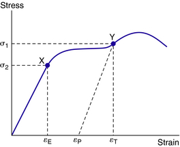
 (3-5)
(3-5)where εT = total strain under load, εP = plastic (or permanent) strain, and εE = elastic strain.
Yield point
Yield point (point b on the stress–strain diagram of Fig. 3-12) refers to that point at which a marked increase in strain occurs without a corresponding increase in stress. The horizontal portion of the stress–strain curve (b-c-d in Fig. 3-12) indicates the yield stress corresponding to this yield point. The yield point is the “knee” in the stress–strain curve for a material and separates the elastic from the plastic portions of the curve.
Tensile strength
The tensile strength of a material is obtained by dividing the maximum tensile force reached during the test (e on the stress–strain diagram in Fig. 3-12) by the original cross-sectional area of the test specimen. Practical application of the maximal tensile force is minimal because devices are never designed to be loaded to this value.
Toughness and ductility
The area under the curve to the point of maximum stress (a-b-c-d-e in Fig. 3-12) indicates the toughness of the material, or its ability to withstand shock loads before rupturing. The supporting arms of a car bumper are an example of where toughness is of great value as a mechanical property. Ductility is the ability of a material to sustain large permanent deformations in tension, as drawing a rod into a wire. The distinction between ductility and toughness is that ductility deals only with the ability to deform, whereas toughness considers both the ability to deform and the stress developed during the deformation. The requirement for plastic deformation in sidebars is weighed against the ability of the sidebars to resist large rapid loads and even the forces required by the practitioner to be able to deform them.
Thermal stress
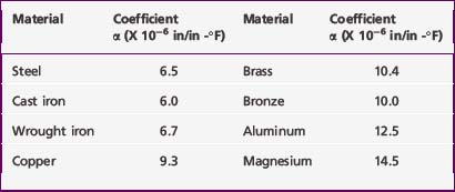
The influence of temperature change is noted through the medium of the coefficient of thermal expansion α, which is defined as the unit strain produced by a temperature change of one degree. This physical constant is a mechanical property of each material. Values of α for several materials are given in Table 3-3.
 (3-6)
(3-6)If the heated rod is compressed back to its original length, then it will experience compression as given by Equation 3-4:
 (3-7)
(3-7)Combining Equations 3-6 and 3-7 and solving for stress, σ = F/A, gives:
 (3-8)
(3-8)Equation 3-8 allows the calculation of stress in a rod as a function of the increase in temperature ΔT, the modulus of elasticity E (Table 3-1), and the coefficient of thermal expansion α (Table 3-2). The concept of change in dimension as the result of temperature rise is illustrated in Example 1 in the Appendix.
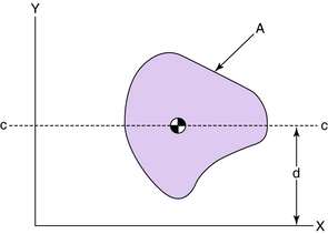
Centroids and center of gravity
For an object of uniform density, the term center of gravity is replaced by the centroid of the area. The centroid of an area is defined as the point of application of the resultant of a uniformly distributed force acting on the area. An irregularly shaped plate of material of uniform thickness t is shown in Fig. 3-17. Two elemental areas (a and b>) are shown with centroids (x1,y1) and (x2,y2), respectively. If the large, irregularly shaped plate is divided into small elemental areas, each having its own centroid, then the centroid for the irregularly shaped plate is (x,y), where:
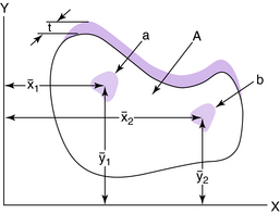


and


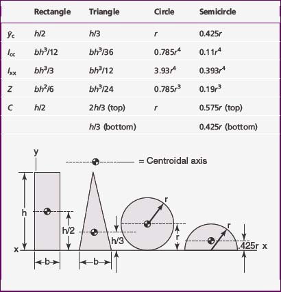
The y-centroids for several common geometric shapes are given in Table 3-3. The general equations for the x– and y-components of the centroid are given in Example 2 in the Appendix.
Moment of inertia
The moment of inertia of a finite area about an axis in the plane of the area is given by the summation of the moments of inertia about the same axis of all elements of the area contained in the finite area. In general, the moment of inertia is defined as the product of the area and the square of the distance between the area and the given axis. The moments of inertia about the centroidal axes Icc of a few simple but important geometric shapes are determined by integral calculus and are given in Table 3-3. Although Young’s modulus is an indication of the strength of the material, the moment of inertia is an indicator of the strength of a particular shape about the aspect in which it will be loaded. This is a highly important parameter for the practitioner to know because he or she often will be able to influence the shape.
Parallel axis theorem
When the moment of inertia has been determined with respect to a given axis, such as the centroidal axis, the moment of inertia with respect to a parallel axis can be obtained by the parallel axis theorem, provided one of the axes passes through the centroid of the area. The parallel axis theorem states that the moment of inertia with respect to any axis is equal to the moment of inertia with respect to a parallel axis through the centroid added to the product of the area and the square of the distance between the two axes (Fig. 3-18):

 (3-9)
(3-9)where Ixx = moment of inertia about x-axis, Icc = moment of inertia about centroid, A = area, and d = distance between axes.
Stresses in beams
If forces are applied to a beam as shown in Fig. 3-19, downward bending of the beam occurs. Imagine a beam is composed of an infinite number of thin longitudinal rods or fibers. Each longitudinal fiber is assumed to act independently of every other fiber (i.e., there are no lateral stresses [shear] between fibers). The beam of Fig. 3-19 will deflect downward and the fibers in the lower part of the beam undergo extension, whereas those in the upper part shorten. The changes in the lengths of the fibers set up stresses in the fibers. Those that are extended have tensile stresses acting on the fibers in the direction of the longitudinal axis of the beam, whereas those that are shortened are subject to compression stresses.
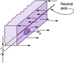
For any beam having a longitudinal plane of symmetry and subject to a bending torque T at a certain cross-section, the normal stress σ, acting on a longitudinal fiber at a distance y from the neutral axis of the beam (Fig. 3-20), is given by:
 (3-10)
where I = moment of inertia of the cross-sectional area about the neutral or centroidal axis in inches4.
These stresses vary from zero at the neutral axis of the beam (y = 0) to a maximum at the outer fibers (Fig. 3-20). These stresses are called bending, flexure, or fiber stresses.
Section modulus
 (3-11)
The ratio I/c is called the section modulus and usually is denoted by the symbol Z. The section moduli for the shapes given in Table 3-3 are obtained by dividing the moment of inertia about the centroidal axis by the length of the centroid. For example, the moment of inertia for a rectangle about its centroidal axis is bh3/12 and the length of the centroid is h/2; therefore, the section modulus is bh2/6. Section moduli are given in Table 3-3.
Beam torque
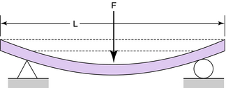
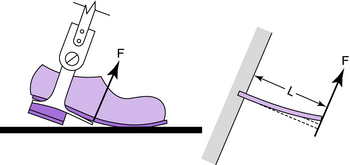
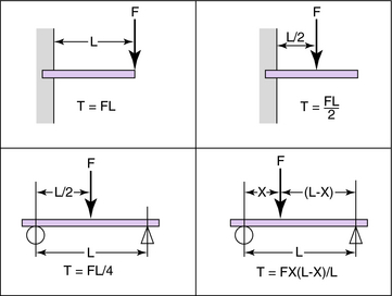
Most structural elements in orthoses can be represented by either a cantilever beam loaded transversely with a perpendicular force at the end (e.g., a stirrup in terminal stance; Fig. 3-21) or a beam freely supported at the ends and centrally loaded (e.g., KAFO prescribed to control valgum; Fig. 3-22).
The maximum torque in cantilevered (Fig. 3-21) and freely supported (Fig. 3-22) beams is given by:
 (3-12)
 (3-13)
Figure 3-23 gives the maximum torque for a few simple beams. If more than one external force acts on a beam, the bending torque is the sum of the torques caused by all the external forces acting on either side of the beam. Subsequently and not surprisingly, device failures commonly occur at the corresponding point of maximum torque (bending moment).
Beam stress
The stress in a cantilevered or freely supported beam now can be determined by substituting Equation 3-12 or 3-13 into Equation 3-11, which gives:
 (3-14)
 (3-15)
 (3-16)
 (3-17)
Beam deflection
Deflection theory provides a technique of analysis for evaluating the nature and magnitude of deformations in beams. The cantilevered beam (Fig. 3-24) carries a concentrated downward load F at the free end. A cantilevered beam is, by definition, rigidly supported at the other end. The general expression for the downward deflection y, anywhere along the length (x-axis) of the beam, is given by:
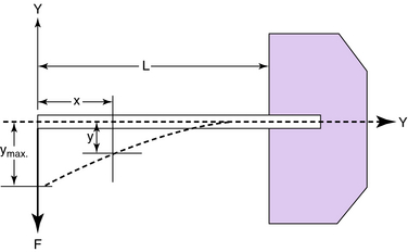
 (3-18)
The maximum deflection of the cantilevered beam (ymax) occurs at the free end when x = 0:
 (3-19)
The general expression for the deflection of the freely supported beam with the midspan load (Fig. 3-25) is given by:
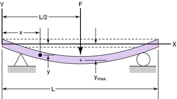
 (3-20)
The maximum deflection of the freely supported beam (ymax) occurs at the midspan when x = L/2:
 (3-21)
The negative sign in Equations 3-19 and 3-21 indicates that the maximum deflection is downward from the unloaded position. Example 4 in the Appendix provides an illustration of calculating KAFO stress and deflection using the concepts of moment of inertia and centroid.
Metals
Crystallinity
Common iron is an example of one of many metals that may exist in more than one lattice form:
A metal in the liquid state is noncrystalline, and the atoms move freely among one another without regard to interspatial distances. The internal energy possessed by these atoms prevents them from approaching one another closely enough to come under the control of their attractive electrostatic fields. However, as the liquid cools and loses energy, the atoms move more sluggishly. At a certain temperature, for a particular pure metal, certain atoms are arranged in the proper position to form a single lattice typical of metal. The temperature at which atoms begin to arrange themselves in a regular geometric pattern (lattice) is called the freezing point. As heat is removed from metal, crystallization continues, and the lattices grow about each center. This growth continues at the expense of the liquid, with the lattice structure expanding in all directions until development is stopped by interference with other space lattices or with the walls of the container. If a space lattice is permitted to grow freely without interference, a single crystal is produced that has an external shape typical of the system in which it crystallizes.
Crystallization centers form at random throughout the liquid mass by the aggregation of a proper number of atoms to form a space lattice. Each of these centers of crystallization enlarges as more atoms are added, until interference is encountered. A diagrammatic representation of the process of solidification is shown in Fig. 3-29. In this diagram, the squares represent space lattices. In A, crystallization has begun at four centers.
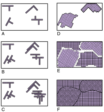
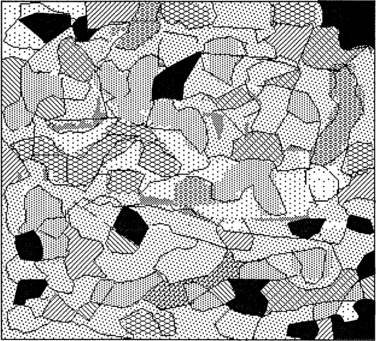
As crystallization continues, more centers appear and develop with space lattices of random orientation. Successive stages in the crystallization are shown by B, C, D, E, and F. Small crystals join large ones, provided they have about the same orientation (i.e., their axes are nearly aligned). During the last stages of formation, crystals meet, but there are places at the surface of intersections where development of other space lattices is impossible. Such interference accounts for the irregular appearance of crystals in a piece of metal that is polished and etched (Fig. 3-30).
Slip planes
When a force is applied to a crystal, the space lattice is distorted as evidenced by a change in the crystal’s dimensions. This distortion causes some atoms in the lattice to be closer together and others to be farther apart. The magnitude of the applied force necessary to cause the distortion depends on the forces that act between the atoms in the lattice and tends to restore it to its normal configuration. If the applied force is removed, the atomic forces return the atoms to their normal positions in the lattice. Cubic patterns (lattices) characterize the more ductile or workable materials. Hexagonal and more complex patterns tend to be more brittle or more rigid. The force required to bring about the first permanent displacement corresponds to the elastic limit. This permanent displacement, or slip, occurs in the lattice on specified planes called slip planes. The ability of a crystal to slip in this manner without separation is the criterion of plasticity. Practically all metals are plastic to a certain degree. During plastic deformations, the lattice undergoes distortion, thus becoming highly stressed and hardened.
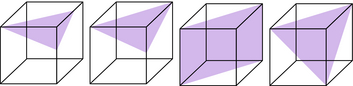
A particular characteristic of crystalline materials is that slip is not necessarily confined to one set of planes during the process of deformation. Some common planes of slip in the simple cubic system are shown in Fig. 3-31.
Mechanical properties
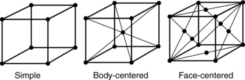
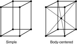
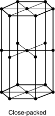
The mechanical properties of metals depend on their lattice structures. In general, metals that exist with the face-centered cubic structure are ductile throughout a wide range of temperatures. Metals with the close-packed hexagonal type of lattice (Fig. 3-28) are appreciably hardened by cold working, and plastic deformation takes place most easily on planes parallel to the base of the lattice.
Plasticity
A simple two-dimensional representation of a cubic crystal lattice in an unstrained condition is represented by A in Fig. 3-32. If a shearing force within the elastic range is applied, the lattice is uniformly distorted as in B, with the extent of distortion proportional to the applied force.
Similar relations exist for other pure metals.
Imperfections of many kinds, such as flaws in the regularity of the crystal lattice, microcracks within a grain, shrinkage voids, nonmetallic inclusions, rough surfaces, and notches of all kinds, may localize and intensify stresses. Many impurities owe their potency to a high degree of insolubility in the solid matrix coupled with high solubility in the fusion. This permits their freezing out relatively late in the solidification process, as concentrates or films between the grains, thus serving as effective internal notches. The great weakening effect of graphite flakes in cast iron is an example.


