Computed Tomography Scanner Technology

The original CT scanners were introduced for clinical medical imaging in 1972. These first-generation CT scanners consisted of a gantry in which x-rays produced at one end traveled through the patient and then to a detector 180 degrees away, which would measure the amount of attenuation of the x-ray beam. The x-ray source and the detector would translate around the patient, and the information from this slice would be converted to a gray-scale, cross-sectional image with the use of a computerized filtered back projection. In this image, each pixel represented a measurement of the mean x-ray attenuation. Structures that attenuate x-rays more than water (i.e., cortical bone and muscle) will have positive CT numbers or Hounsfield units, whereas structures that attenuate x-rays less than water (i.e., air and fat) have negative CT Hounsfield units. High-attenuation structures would appear white whereas at the opposite end of the scale would appear black. The imaging of the patient would take up to 30 minutes as the patient moved through the gantry in a stepwise manner, 1 cm at a time, until the region of interest was imaged. The next-generation CT scanners increased the number of detectors in one row so that the x-ray beam fanned out from its source and hit multiple detectors at one time; this reduced imaging time. Additional improvements in 1989 included the spiral or helical scanning of the patient so that the patient would move continuously through the gantry; this again reduced imaging time. With this technique, a series of images could be obtained during the holding of a single breath.

The next generation of CT scanners then added rows of detectors; this technology is referred to as multislice CT, multichannel CT, or multidetector CT (MDCT). The initial MDCT scanners introduced in 1992 could image only two slices at the same time, but this number has since increased; currently available commercial scanners can image 64, 128, or even 256 rows or slices. There are several benefits of such MDCT scanners. One significant benefit is the markedly reduced time that it takes to acquire images; an entire extremity can be imaged with this type of CT with less than 1 minute of imaging time. Another benefit is that high x-ray tube current, which is measured as milliampere-seconds, can be achieved to allow imaging through metal hardware; however, this advantage is offset by the increased radiation dose required. Another significant benefit is that slice thicknesses of less than 1 mm are now attainable, which allows for high-resolution imaging and, more important, for high-resolution reformatted images in any plane.

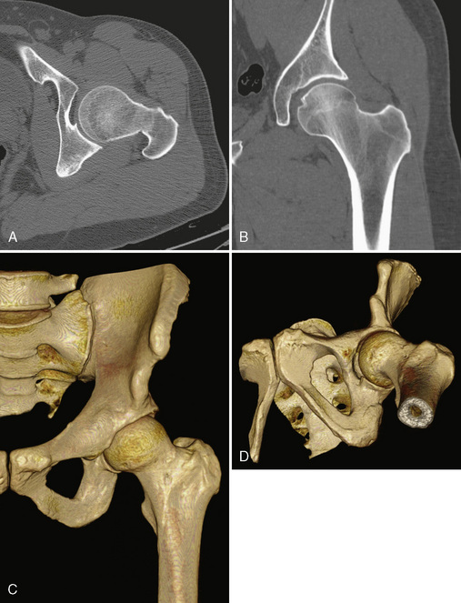
Two- and Three-Dimensional Reformatted Computed Tomography Images

Before the invention of MDCT scanners, the ability to reformat the original axial data set into other imaging planes was markedly limited. The resulting images were often distorted with a venetian-blind effect with steplike contours, and thus they were of limited diagnostic quality. With the advent of MDCT scanners, however, this has dramatically improved. The reason behind this is the concept of isotropic imaging. If a volume of tissue (i.e., a voxel) is imaged at a very small quantity such that the length, width, and height of the volume are equal, then a reformatted image retains high resolution as compared with the axial images (Figure 5-1, A and B). It is possible to obtain these images with the use of MDCT scanners with 16 or more detector rows that allow for a slice thickness of less than 1 mm. A standard protocol for the imaging of any extremity with CT is to reconstruct the original data at a slice thickness of less than 1 mm with 50% overlap of each slice and to then produce two-dimensional reformatted images 1- to 2-mm thick in the axial, sagittal, and coronal planes. MDCT scanners now have several options or tools that allow for three-dimensional reformatted imaging and surface rendering. At an independent workstation, these data can be manipulated to remove overlying soft tissues, osseous structures, or hardware and to produce a rotating volumetric data set (Figure 5-1, C and D).

Figure 5–1 Normal CT of the hip. A, Axial CT image. B, Coronal multiplanar reformatted CT image. C and D, Surface rendering three-dimensional CT images show a normal left hip.

Radiation Exposure

Although imaging quality and resolution improve with the use of MDCT, one must understand that this is at the expense of radiation dose. The effective radiation dose takes into account the tissue being irradiated and the type of radiation, and it is measured in units of rem or sievert (Sv), with 100 rem being equal to 1 Sv. The effective patient dose for CT of the pelvis is approximately 3 mSv to 4 mSv. To put this into perspective, a single posteroanterior chest radiograph is approximately 0.02 mSv, and the average annual background radiation dose in the United States is 3.6 mSv. A statistically significant increase in cancer is seen among individuals who have been exposed to 50 mSv or more; this was determined on the basis of a study of atomic bomb survivors in Japan. The radiation dose from CT is not insignificant, and this becomes even more problematic in the patient who is young or potentially wants to bear children. As with any imaging study, the medical necessity of the test should be weighed against the risks of the examination.

Femoroacetabular Impingement and Computed Tomography Arthrography

Impingement between the proximal femur and the acetabulum may be classified as cam type, pincer type, or mixed type. With the cam type of femoroacetabular impingement (FAI), a nonspheric femoral head with an abnormal contour of the femoral head–neck junction directly impinges on the acetabulum and labrum with flexion, adduction, and internal rotation of the hip. Proposed causes for this type of impingement include prior slipped capital femoral epiphysis, prior trauma, and growth disturbance with distortion of the physis. With the pincer type of FAI, there is abnormal contact between the acetabulum and the proximal femur from acetabular causes (e.g., retroversion, protrusio, acetabular rim prominence) or femoral causes (e.g., coxa magna, coxa profunda).

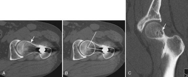
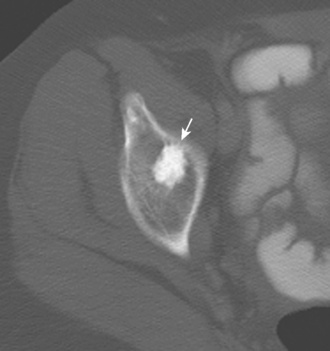
Many of the imaging features of FAI include bony abnormalities. Although magnetic resonance imaging (MRI) has also been used to demonstrate these findings, CT is well suited for characterizing bone abnormalities (Figure 5-2, A). With the cam type of FAI, the abnormal contour at the femoral head–neck junction is measured as the alpha angle, which indicates where the bone contour of the femoral head extends beyond the confines of the femoral head. An angle of more than 55 degrees measured on a sagittal–oblique image parallel to the femoral neck is considered abnormal and correlates with the cam type of FAI (Figure 5-2, B). Other bony changes associated with the cam type of FAI are well demonstrated with CT, including fibrocystic changes at the anterosuperior femoral neck (Figure 5-2, C). Such fibrocystic changes are more common among patients with FAI, and they may be directly caused by impingement. CT has an advantage over radiography for showing such cortical changes. Other radiographic signs of the cam type of FAI, such as the abnormal contour of the femoral head–neck junction (pistol grip deformity), are also well delineated on CT, because patient positioning may not optimally profile the bone contour deformity.

Figure 5–2 Femoroacetabular impingement, cam type. A, Axial CT image shows abnormal contour (arrow) at the femoral head–neck junction. B, Abnormal alpha angle, which measures more than 55 degrees, and incidental proximal femur intramedullary nail. C, Coronal multiplanar reformatted CT image from a different patient shows cortical defects with sclerotic margins (arrow).

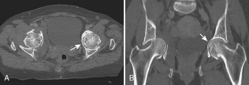
With regard to CT of the pincer type of FAI, bony abnormalities such as acetabular protrusion (Figure 5-3) and acetabular retroversion may be demonstrated. When assessing for acetabular retroversion on radiography, the crossover sign (i.e., the anterior acetabular wall projects lateral to the posterior acetabular wall) may be affected by patient positioning. CT avoids this pitfall by directly measuring the acetabular version, which is described as 23 degrees in females (range, 10 to 37 degrees) and 17 degrees in males (range, 4 to 30 degrees). A retroverted acetabulum is associated with the pincer type of FAI and with hip osteoarthrosis. CT is also effective for measuring anterior and posterior acetabular sector angles in the setting of hip dysplasia.

Figure 5–3 Femoroacetabular impingement, pincer type. A, Axial and B, coronal multiplanar reformatted CT images show (arrow) left acetabular protrusio. Note the right acetabular fracture.

One of the benefits of MRI and, more important, of MR arthrography for the assessment of FAI is that cartilage abnormalities may also be diagnosed in addition to the previously described bony abnormalities. Although the evaluation of the cartilaginous structures is limited with routine CT, the use of intra-articular iodinated contrast in conjunction with CT (or CT arthrography) can effectively diagnose labral and hyaline cartilage abnormalities, which are seen with FAI. With the use of isotropic imaging that can produce a submillimeter slice thickness, CT arthrography can diagnose a labral tear with 97% sensitivity, 87% specificity, and 92% accuracy. Similarly, CT arthrography can diagnose articular cartilage disorders with 88% sensitivity, 82% specificity, and 85% accuracy. In the setting of hip dysplasia, labral and hyaline cartilage abnormalities commonly coexist. The use of radial reformatted CT is also possible with submillimeter slice thicknesses and isotropic imaging.

Hip Trauma

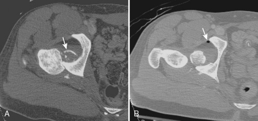
CT is often used to evaluate the hip and acetabulum after hip dislocation and other pelvic trauma (Figures 5-3 and 5-4). When an acetabular fracture is identified by radiography, CT can further characterize the fracture pattern with the use of multiplanar reformatted images and three-dimensional surface rendering (see Figure 5-3). Associated abnormalities such as intra-articular bodies and pelvic hematoma are also well demonstrated with CT. After hip dislocation, CT demonstrates the position of the femoral head and the coexisting femoral head fracture (see Figure 5-4, A). A sign of prior hip dislocation on CT is the presence of a bubble of gas, which is most commonly seen at the anterior aspect of the hip joint (see Figure 5-4, B).

Figure 5–4 Femoral head fracture and dislocation. A, Axial CT image shows a posterior dislocation of the right hip with a comminuted femoral head fracture (arrow). B, Axial CT image with soft-tissue windows shows an air bubble (arrow) anterior to the hip joint.

It is important to understand the advantages and disadvantages of CT for the evaluation of fracture. CT is most accurate for demonstrating fractures of cortical bone (Figure 5-5, A). In an osteopenic patient in whom the cortex is thin, accuracy will decrease, especially when the fracture is not displaced. This becomes even more problematic for the diagnosis of an intramedullary fracture. In an osteopenic patient in whom the trabeculae are thin or resorbed, a fracture may not be apparent on CT. MRI has been shown to be more accurate than CT for the evaluation of proximal femur fractures in patients more than 50 years old where CT led to a misdiagnosis in 66% of patients. In addition, CT may not show the entire intramedullary extent of a presumed isolated greater trochanteric fracture. As a general rule, CT is most effective for diagnosing fractures of cortical bone in younger patients, and it is relatively limited with regard to intramedullary fractures among the elderly (e.g., insufficiency-type stress fractures). By contrast, a chronic-fatigue–type stress fracture is well demonstrated with CT given the associated sclerosis (Figure 5-5, B).

Figure 5–5 Stress fracture, fatigue type. A, Axial CT image shows an acute cortical fracture as linear low attenuation (arrow). B, Coronal multiplanar reformatted CT image from a different patient shows a chronic cortical fracture (arrow) as a linear low-attenuation fracture line and a thickened high-attenuation cortex.

Hip Arthroplasty

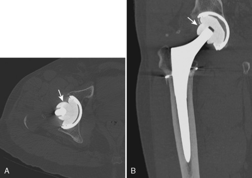
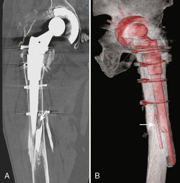
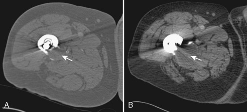
Although radiography is the imaging method of choice for the routine evaluation of the hip after arthroplasty, CT does have a role in specific scenarios, such as the evaluation of infection, osteolysis, and component position. The technical advance that permits for the CT evaluation of metal with reduced artifact is MDCT, which allows increased x-ray tube current to image through metal. The individual components of an arthroplasty as well as the adjacent soft tissues and bone can be visualized with CT (Figure 5-6). This is helpful for displaying fracture (Figure 5-7) and for the diagnosis of soft-tissue infection adjacent to a prosthesis (Figure 5-8). In the presence of component wear and particle disease, CT can directly show the polyethylene component wear as well as the adjacent osteolysis (Figure 5-9). Although radiography adequately screens for osteolysis, CT more accurately measures the volume of osteolysis. CT can also be used to measure component version after hip arthroplasty.

Figure 5–6 Total hip arthroplasty, normal. A, Axial and B, coronal multiplanar reformatted CT images show a cementless total hip arthroplasty. Note the ceramic acetabular and femoral head (arrow) surfaces, which are lower in attenuation as compared with metal.

Figure 5–7 Component failure, total hip arthroplasty revision. A, Coronal multiplanar reformatted CT image, and B, three-dimensional rendering with partially transparent bone and red-colored metal shows femoral component failure (arrow).

Figure 5–8 Infection, total hip arthroplasty. Axial CT images after intravenous contrast in A, bone, and B, soft-tissue windows, show cortical destruction and adjacent soft-tissue fluid collection (arrow).

Figure 5–9 Particle disease, total hip arthroplasty. Axial CT image in soft-tissue windows shows focal areas of bone lysis (arrows) of the acetabulum replaced with soft-tissue attenuation.

Miscellaneous Hip Abnormalities

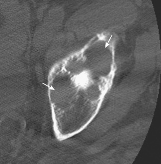
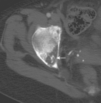
Other hip disorders that involve the bone or that produce calcification or ossification can be evaluated with CT. Primary synovial osteochondromatosis is a benign neoplastic condition in which hyaline cartilage nodules form in the subsynovial tissue of a single large joint. If these nodules ossify, they are readily demonstrated on CT as multiple uniform ossific bodies in the joint (Figure 5-10). Secondary osteoarthrosis and associated erosions may also be present. The hip is the second most common joint affected by this condition, after the knee.

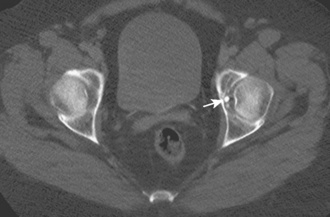
Figure 5–10 Synovial osteochondromatosis. Axial CT image shows several ossified cartilaginous bodies (arrow).

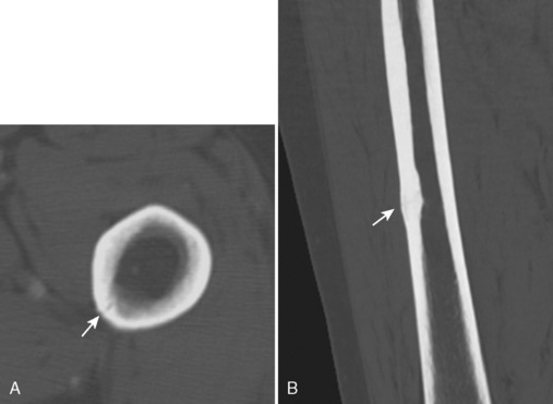
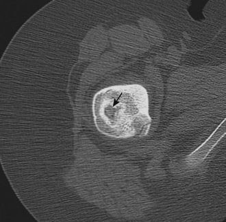
Osteoid osteoma is a benign bone lesion of uncertain origin that involves a vascularized nidus being present within the bone, typically the cortex. When this occurs in an extra-articular location, the nidus is associated with significant sclerosis and periostitis (Figure 5-11). When it is intra-articular, there is associated effusion and synovitis. CT shows the nidus as a round area of low attenuation with surrounding sclerosis that may calcify. CT can be used to effectively guide the percutaneous thermoablation of osteoid osteomas.

Figure 5–11 Osteoid osteoma. Axial CT image shows a low-attenuation nidus (arrow) with partial calcification. Note the surrounding high-attenuation sclerosis.

CT may also be used to characterize other bone abnormalities. When a sclerotic focus is present within the bone, CT can show the uniform sclerotic density and spiculated margins that are typical of a bone island or enostosis (Figure 5-12). The calcified matrix of a chondroid tumor such as chondroblastoma or chondrosarcoma (Figure 5-13) or the ossified matrix of an osteosarcoma can be demonstrated with CT, which assists with the characterization of a primary bone tumor. CT is the typical imaging method used for the percutaneous imaging-guided biopsy of a bone tumor that involves the pelvis or the proximal femur.

Figure 5–12 Bone island (enostosis). Axial CT image shows a high-attenuation sclerotic focus with speculated margins (arrow).

Figure 5–13 Chondrosarcoma. Axial CT image shows low-attenuation bone destruction with a calcified matrix (arrow).

Ultrasound Technology

Ultrasound is a unique imaging method in that it does not involve ionizing radiation but rather makes use of sound waves to produce images. A sound wave is transmitted from the ultrasound transducer, which is placed on the skin surface with acoustic coupling gel. The sound wave propagates through the soft tissues, interacts at soft-tissue interfaces, and then returns to the transducer, where the sound waves are converted into an image. At interfaces where there is a significant difference in impedance, nearly all of the sound waves are reflected back to the transducer, which produces a bright echo that is displayed on the image. The echoes on the ultrasound image are described as hyperechoic (bright echo), isoechoic (equal echo), hypoechoic (low echo), or anechoic (no echo) as compared with the surrounding tissues. Cortical bone is hyperechoic with shadowing, tendon is hyperechoic and fibrillar, muscle is hypoechoic with interspersed hyperechoic fibroadipose septae, and simple fluid is anechoic. An important technical option on most ultrasound machines is color or power Doppler imaging, which shows blood flow as color on the ultrasound image.