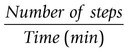
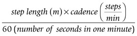
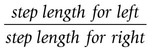
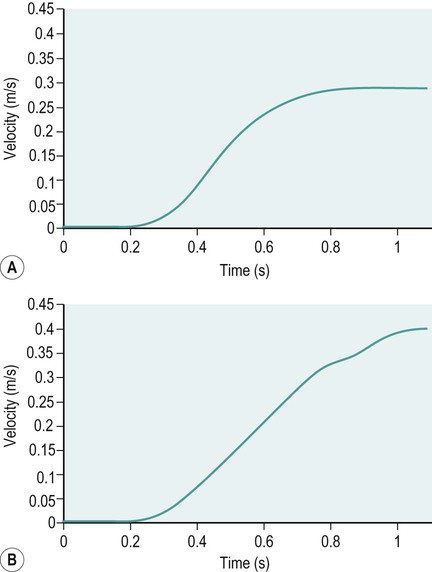
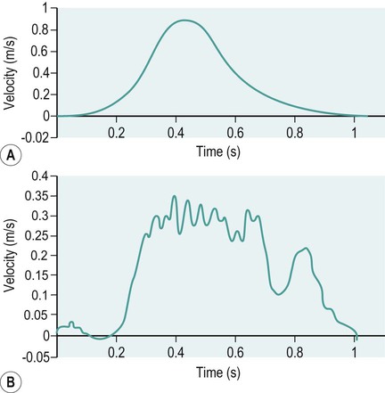
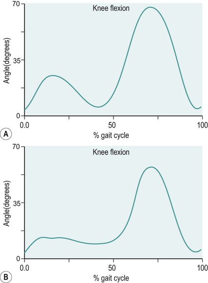
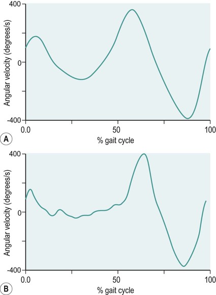
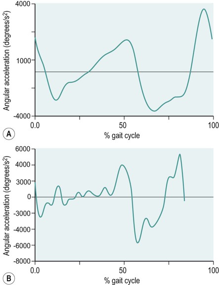
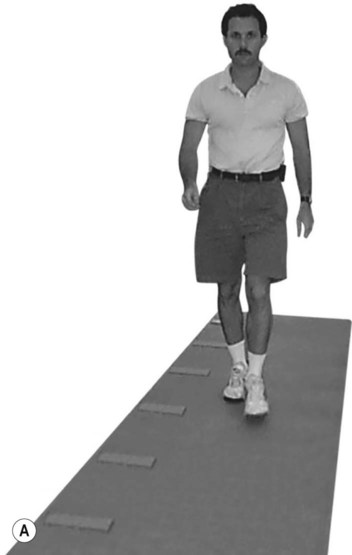
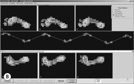
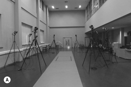
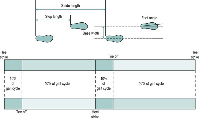
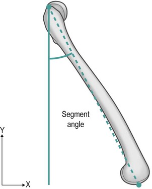
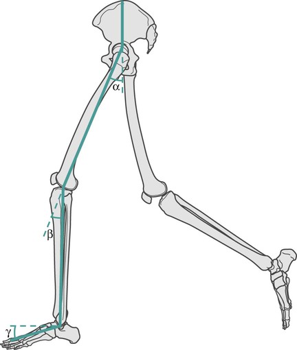
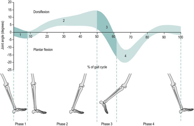
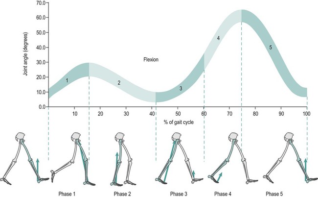
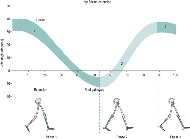
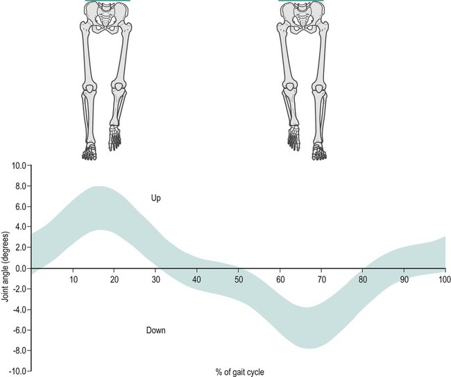
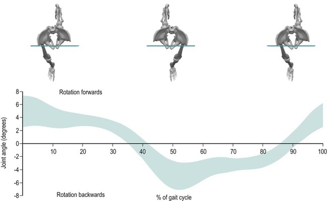
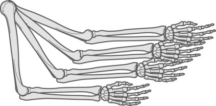
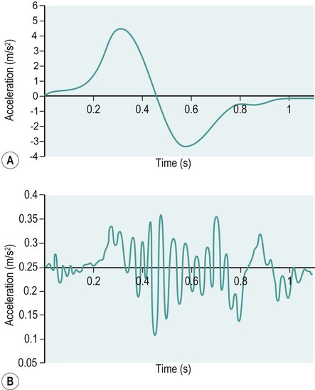
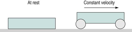
This chapter will take you through an introduction to clinical gait analysis, definitions and detailed descriptions of the movement and force patterns found during walking, and the mathematical basis of how joint movement, muscle forces and power may be calculated. More information about clinical biomechanics is available in the textbook Biomechanics in Clinic and Research: An Interactive Teaching and Learning Course (Richards 2008). In 1953, Saunders and co-workers referred to the major determinants in normal gait and applied these to the assessment of pathological gait. Inman (1966, 1967) and Murray (1967) both published detailed analyses on the kinematics and conservation of energy during human locomotion, and these are resources still frequently referred to. Inman et al. (1981) later published Human Walking, a comprehensive textbook on human locomotion. Brand and Crowninshield (1981) highlighted the distinction between the use of biomechanical techniques to ‘diagnose’ or ‘evaluate’ clinical problems. The authors stated: ‘Evaluate, in contrast to diagnose, means to place a value on something. Many medical tests are of this variety and instead of distinguishing diseases, help determine the severity of the disease or evaluate one parameter of the disease. Biomechanical tests at present are of this variety’. Brand and Crowninshield also gave a guide of six requirements for tools used in patient evaluation: 1. The measured parameter(s) must correlate well with the patient’s functional capacity 2. The measured parameter must not be directly observable and semi-quantifiable by the physician or therapist 3. The measured parameters must clearly distinguish between normal and abnormal 4. The measurement technique must not significantly alter the performance of the evaluated activity 5. The measurement must be accurate and reproducible 6. The results must be communicated in a form which is readily identifiable. Brand and Crowninshield stated: ‘It is clear to us that most methods of assessing gait do not meet all of these criteria. We believe that it is for this reason that they are not widely used.’ Advances in biomechanical assessment in the last 30 years have been considerable. The description of normal gait in terms of movement and forces about joints is now commonplace. The relationship between normal gait patterns and normal function is also well supported in both scientific articles and textbooks (Bruckner 1998; Rose and Gamble 2005; Perry 2010, Levine et al. 2012). This allows deviations in gait patterns to be studied in relation to changes in function in subjects with particular pathologies. It is possible for a clinician or physician to subjectively study gait, but the value and repeatability of this type of assessment is questionable owing to poor inter- and intra-tester reliability (Pomeroy et al. 2003). It is impossible for one individual to study simultaneously, by observation alone, the movement pattern of all the main joints involved during an activity like walking. Studying movement patterns using objective motion analysis allows information to be gathered simultaneously with known accuracy and reliability. In this way, changes in movement patterns owing to intervention by physical therapists and surgeons may be assessed unequivocally. Most motion analysis systems now report on the joint kinematics of the recorded individual and also contain the mean for normal data on the same graph, allowing a direct comparison of the individual’s movement pattern in relation to a predefined normal. Such information is also available in Clinical Gait Analysis: Theory and Practice (Kirtley 2005). Patrick (1991) reviewed the use of movement analysis laboratory investigations in assisting decision-making for the physician and clinician. Patrick concluded that the reasons for the use of such facilities not being widespread were owing to: • the time of analysis being considerable; • bioengineers designing systems and presenting results for researchers and not clinicians; • a lack of understanding by physicians and clinicians of applied mechanics and its relevance to assessment of treatment outcome. A common argument against movement analysis laboratories has been cost. The cost of movement analysis equipment and its potential use in the clinical setting has been reported (Bell et al. 1996). Indeed, a broader question could be put to any clinical assessment or treatment that requires the use of technology. One example of this is the relative cost of radiography to movement analysis equipment, which, in comparison, is modest. Gage (1994) claimed that gait analysis costs are comparable with magnetic resonance imaging (MRI) or computed axial tomography (CAT) scans. Gage also stated that the use of movement analysis, as a detailed form of assessment, may have wider cost benefits and improve clinical services more than first realised. Bell et al. (1995) highlighted the use of a holistic approach to motion analysis, which included muscle performance, joint range of motion, kinematic and kinetic parameters of gait. This holistic approach may be applied to many pathologies to give a detailed assessment of pathology and the subsequent effects of treatment. • The stance phase can be subdivided into: heel strike, foot flat, mid-stance, heel off and toe off. • The swing phase can be subdivided into: early swing, mid-swing and late swing. We can display spatial parameters of foot contact during gait as a series of footprints (Figure 15.1). These can also be defined as follows: • step length – the distance between two consecutive heel strikes; • stride length – the distance between two consecutive heel strikes by the same leg; • foot angle or angle of gait – the angle of foot orientation away from the line of progression; • base width or base of gait – the medial lateral distance between the centre of each heel during gait. We can display temporal parameters of heel strike and toe off pictorially (Figure 15.1). These can also be defined as follows: • step time – the time between two consecutive heel strikes; • stride time – the time between two consecutive heel strikes by the same leg, one complete gait cycle; • single support – the time over which the body is supported by only one leg; • double support – the time over which the body is supported by both legs; • swing time – the time taken for the leg to swing through while the body is in single support on the other leg; • total support – the total time a foot is in contact with the ground during one complete gait cycle. Two other parameters may easily be calculated using this information: cadence and velocity. The cadence is the number of steps taken in a given time, usually steps per minute. Velocity may be calculated by: Symmetry can also be assessed by dividing the value of a parameter found for the left over that of the right: These parameters, although simple, can be a very useful means of outcome assessment. It must be noted, however, that these may not always be appropriate for some more complex pathological gait patterns (Wall et al. 1987). For example, the features of Parkinsonian gait can include a reduction in stride length and velocity, and an increase in base width. However, this results in a characteristic shuffling gait which makes it hard to determine the events of heel strike and toe off. For further information on Parkinson’s disease, please refer to Chapter 24. Human walking allows a smooth and efficient progression of the body’s centre of mass (Inman 1967). To achieve this there are a number of different movements of the joints in the lower limb. The correct functioning of the movement patterns of these joints allows a smooth and energy efficient progression of the body. The relationship between the movements of the joints of the lower limb is critical. If there is any deviation in the coordination of these patterns the energy cost of walking may increase and the shock absorption at impact and propulsion may not be as effective. Segment angles are defined as the angle of body segments away from the vertical axis (Figure 15.2). Segment angles can be calculated by knowing the co-ordinates of the proximal and distal ends of a body segment in a particular plane. The angle can then be found using trigonometry. A joint angle is defined as the angle between the line of the proximal and distal segments of a joint. Figure 15.3 shows the hip, knee and ankle joint angles (α,β,γ). The ankle joint angle is defined by the foot with respect to a line 90 degrees to the tibia, with dorsiflexion defined as a positive angle and plantar flexion as a negative angle. The knee joint angle is defined by the long axis of the tibia with respect to the long axis of the femur, with full extension defined as zero degrees and movement into flexion being positive. The hip joint angle is defined by the long axis of the femur with respect to the pelvis, with flexion defined as positive and extension negative. The range of motion that occurs in walking varies between 20 degrees and 40 degrees, with an average value of 30 degrees. However, this does not tell us how the motion of the ankle varies throughout gait. During gait the ankle has four phases of motion (Figure 15.4). During gait the knee joint moves in the sagittal, transverse and coronal planes. However, the majority of the motion of the knee joint is in the sagittal plane, which involves the flexion and extension of the knee joint. The flexion and extension of the knee joint is cyclic and varies between 0 and 70 degrees, although there is some variation in the exact amount of peak flexion occurring. These differences may be related to differences in walking speed, subject individuality and the landmarks selected to designate limb segment alignments. There are five phases (Figure 15.5). The motion of the hip joint is relatively simple (Figure 15.6). Maximum hip flexion occurs during terminal swing (phase 3), this is followed by a slight extension before initial contact, (phase 1). After initial contact (phase 1) the hip then extends as the body moves over the limb at a rate of 150 degrees per second. Maximum hip extension occurs just after opposite foot strike (phase 2), weight is then transferred to the forward limb and the trailing limb begins to flex at the hip. This is the pre-swing period. The toe leaves the ground at 60% of the gait cycle and the hip flexes rapidly at a rate of 200 degrees per second. This can be seen from the slope of the angle against time plot below, to progress the limb forward and prepare for the next initial contact (phase 1). During the early stance phase the contralateral (swing) side of the pelvis drops downward in the coronal plane (Figure 15.7). In order to achieve foot clearance the knee on the contralateral side undergoes rapid flexion. In normal gait the peak pelvic obliquity (drop down) occurs just after opposite toe off, which corresponds to the early stance phase on the weight-bearing limb. During normal level walking the pelvis rotates about a vertical axis alternately to the left and to the right (Figure 15.8). This rotation is usually about four degrees on each side of this central axis – the peak internal rotation occurring at foot strike and the maximal external rotation at opposite foot strike. This rotation effectively lengthens the limb by increasing the step length and prevents excessive drop of the body, making the walking pattern more efficient. Pelvic rotation also has the effect of smoothing the vertical excursion of the body and reducing the impact at foot strike. This graph is drawn from knowing how the linear position of the hand varies over time. Figure 15.9 shows the hand starting at a position zero and moving forwards in a reaching motion. The gradient of the curve indicates the velocity at which the hand is moving throughout the task. Figure 15.10a shows an individual who is pain- and pathology-free and Figure 15.10b shows an individual with a painful, unstable shoulder. Both show a similar pattern; however, the individual with the painful unstable shoulder appears to have a less smooth pattern of movement. We are, however, limited in the measurements we may take from linear displacement graphs; at best we can find the time taken to complete the task and the distance reached with very little information about the performance and quality of the movement during the task. The velocity graph is found by measuring the change in the linear displacement over each successive time interval. The linear velocity graph for the hand of the individual who is pain- and pathology-free shows a bell-shaped curve (Figure 15.11a). Initially, the velocity of the hand is zero; the hand then accelerates to its maximum velocity at approximately the mid-point of the reaching movement. The hand then decelerates as it gets closer to its target; this takes slightly longer than the acceleration phase to ensure control and accuracy of hand positioning. The individual with a painful unstable shoulder (Figure 15.11b) shows a marked difference when considering the linear velocity graph. It shows a rapid acceleration then a continuously varying velocity which is followed by a decrease then an increase in velocity indicating either an unstable or painful part of the movement. The peak velocity may be measured from this graph indicating the level of performance of the task. The unsmooth nature of the pattern gives us a further insight to the control of the task but we cannot measure this directly from the linear velocity graph. The acceleration graph is found by measuring the change in the linear velocity over each successive time interval. The individual who is pain- and pathology-free (Figure 15.12a) shows an initial acceleration peak early in the movement. The acceleration then decreases to zero as the hand reaches its maximum velocity. The hand then goes into a deceleration phase as it reaches its target. The peak deceleration is lower than the acceleration phase, and the deceleration phase lasts for a longer period of time, as shown with the velocity curve; again, this is to ensure controlled accuracy of positioning the hand at the target. The individual with a painful unstable shoulder (Figure 15.12b) shows a marked difference when considering the linear acceleration graph – it shows a rapidly changing graph indicating a lack of smooth controlled movement with no clear acceleration and deceleration period. This lack of smoothness tells us important information about a lack of control which could be owing to poor articulation at the shoulder or poor neuromotor control. During normal walking the motion of the knee joint in the sagittal plane varies between 0 and 70 degrees (Figure 15.13a), although there is some variation in the exact amount of peak flexion occurring. At heel strike, or initial contact, the knee is flexed. After the initial contact there is a controlled increase in knee flexion to about 20 degrees when the knee is flexed under maximum weight-bearing load. During this time the knee extensors are acting eccentrically. After this first peak of knee flexion the knee joint extends this in relation to a smooth, eccentrically controlled movement of the body over the stance limb. The knee undergoes a rapid flexion in preparation for swing phase, sometimes referred to as pre-swing. Toe off marks the start of swing phase which allows the toe to clear the ground. During initial-to-mid-swing the knee continues to flex to a maximum of 65–70°. During late swing, the knee undergoes a rapid extension to prepare for the second heel strike. In the patient with medial compartment knee osteoarthritis (Figure 15.13b), the amount of knee flexion attained during stance phase is significantly lower than that of normal, which could indicate poor eccentric control or a pain avoidance mechanism. The knee then re-extends but not to the same amount as normal – again indicating pain avoidance or reduced control. Swing phase appears to follow a normal pattern of movement but with a reduced amount of knee flexion at mid-swing. During normal walking (Figure 15.14a) the knee flexes to approximately 200 degrees per second during loading, which gives a measure of the eccentric control of the knee during loading. The knee then extends at a rate of approximately 100 degrees per second, which shows a smooth, controlled movement over the stance limb as the body moves forwards. During swing phase the knee flexes and extends with an angular velocity of approximately 400 degrees per second. In the patient with medial compartment knee osteoarthritis (Figure 15.14b) the knee flexes with a reduced angular velocity, therefore the eccentric speed and the control of the knee during loading is reduced. The knee extension velocity is markedly reduced indicating a substantial deficit in the control, or pain avoidance when moving over the stance limb. Interestingly, during swing phase the control of the knee flexion extension appears close to that of normal suggesting that the knee can move freely when not under load. During normal walking (Figure 15.15a) the knee shows a steady pattern of acceleration and deceleration during stance and swing phase. The absence of any rapid changes in acceleration shows that the movement is both smooth and controlled. In the patient with medial compartment knee osteoarthritis (Figure 15.15b) the knee shows several points with rapid changes in acceleration during mid-stance, in particular, as the body moves over the stance limb. This reflects a deficit in the smoothness and control during this period. It is also interesting to note a deficit in smooth movement during swing phase, which had previously gone undetected, indicating that this movement is not as smooth as we previously thought. Often in clinical settings, joint angles are assessed simply using a hand-held goniometer. There are several types of goniometer, all giving a crude, but useful, measure of angles and range of motion. Clinically, the goniometer allows a quick and useful assessment of static angles. However, these devices are of little use when measuring angles dynamically during different movement tasks. Further information on clinical measurements using instrumentation such as the goniometer are available in the handbook A Physiotherapist’s Guide to Clinical Measurement (Fox and Day 2009). Spatial parameters can be measured in a variety of simple ways, including putting ink pads on the soles of the subject’s shoes and walking on paper (Rafferty and Bell 1995), and using marker pens attached to shoes (Gerny 1983). Although very cheap, these systems can require awkward and time-consuming analysis. Temporal parameters can be measured by timing how long it takes an individual to walk a set distance and counting the number of steps it took to cover that distance. However, this will only give average velocity and cadence, and will give no value to the symmetry of these parameters. This technique is extremely susceptible to human error. In the last two decades of the twentieth century advances in computer technology led to the development of a number of instrumented walk mat systems. These allow fast collection of temporal and spatial gait data. Using a computer also allows easier, less time-consuming analysis. These systems include apparatus for step length measurement (Durie and Farley 1980), a system for monitoring the position and time of foot contact during walking (Arenson et al. 1983), using a measuring walkway (Hirokawa and Matsumura 1987), a microcomputer-based system (Crouse et al. 1987) and a walk mat system (Al-Majali et al. 1993). Walk mat systems that do not require any modifications to the footwear are now commercially available. These offer far less interference with the gait cycle. One such system is the GAITRiteTM system, which uses pressure sensor arrays to determine foot position (Figure 15.16). In the late nineteenth century the first motion picture cameras recorded patterns of locomotion in both humans and animals. In 1877, Muybridge demonstrated, using photographs, that when a horse is moving at a fast trot there is a moment when all of the animal’s hooves are off the ground and in 1887 published Animal Locomotion. Muybridge later used 24 cameras to study the movement patterns of a running man and in 1901 published The Human Figure in Motion. Marey, a French physiologist, used a ‘photographic rifle’ to photograph movement of animals in 1873, and in 1882 and 1885 to record displacements in human gait to produce the first stick figure of a runner. In the second half of the twentieth century many systems capable of automated and semi-automated computer-aided motion analysis were developed. One of the first systems to become commercially available was the Ariel Performance Analysis System, which required the operator to manually identify the location of joint centres or passive markers placed on the body used for each frame. Since then, the problems of automatic marker identification have been at the forefront of the development of computer-aided motion analysis. In 1974, SELSPOT became commercially available, which allowed automatic tracking of active light-emitting diode (LED) markers; later OptotrakTM and CODATM used a similar technique. VICON, a camera based system, became commercially available in 1982. Since then, many systems based on television-camera technology have been developed, including the Motion Analysis Corporation system, Elite, and Oqus by QualisysTM (Figure 15.17). If an object is at rest it will stay at rest. If it is moving with a constant speed in a straight line it will continue to do so, as long as no external force acts on it. In other words, if an object is not experiencing the action of an external force it will either keep moving or not move at all (Figure 15.18). This law expresses the concept of inertia. The inertia of a body can be described as being its reluctance to start moving or stop moving once it has started.
Biomechanics
Introduction
Clinical gait analysis
Kinematics
The gait cycle
Spatial and temporal parameters of gait
Spatial parameters
Temporal parameters
Analysis of joint movement during gait
How to find segment angles and joint angles
Motion of the ankle joint
Motion of the knee joint
Motion of the hip joint in the sagittal plane
Motion of the pelvis in the coronal plane (pelvic obliquity)
Motion of the pelvis in the transverse plane (pelvic rotation)
Kinematics of a reaching task
Linear displacement of the hand during reaching with and without shoulder dysfunction
Linear velocity of the hand during reaching with and without shoulder dysfunction
Linear acceleration of the hand during reaching with and without shoulder dysfunction
Kinematics of the knee during walking
Knee angular displacement of normal knee function and medial compartment knee osteoarthritis during walking
Knee angular velocity of normal knee function and a patient with medial compartment knee osteoarthritis during walking
Knee angular acceleration of normal knee function and a patient with medial compartment knee osteoarthritis during walking
Methods of movement analysis
Common clinical tools
Walk mat systems
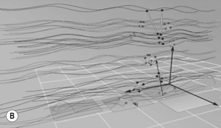
Movement analysis systems
Understanding forces
Forces
Newton’s first law
![]()
Stay updated, free articles. Join our Telegram channel

Full access? Get Clinical Tree


Biomechanics