Maximal Oxygen Consumption

Limitation

The Oxygen Cascade at Maximal Exercise

An Analysis of di Prampero’s Model

Experimental Testing of di Prampero’s Model

An Analysis of Wagner’s Model

Experimental Testing of Wagner’s Model

A Critical Comparison of the Two Models

Of Maximal Oxygen Consumption in Hypoxia

Of Maximal Oxygen Consumption at the End of Bed Rest

Of the Central Governor Hypothesis

Of Measuring ${\varvec{\dot{V}}}\,{\mathbf{O}}_{{{\mathbf{2max}}}}$

Conclusions

References

Abstract

As soon as the concept of maximal oxygen consumption $(\dot{V}\,{\text{O}}_{{2{ \max }}} )$ was created, it was clear that $\dot{V}\,{\text{O}}_{{2{ \max }}}$ was limited somewhere along the respiratory system. The quest for the single factor limiting $\dot{V}\,{\text{O}}_{{2{ \max }}}$ went on for long, with highly contradictory outcomes. The way of looking at $\dot{V}\,{\text{O}}_{{2{ \max }}}$ limitation, however, changed drastically some 30 years ago. The resumption of the oxygen cascade theory as a tool for a holistic description of the respiratory system led to the development of multifactorial models of $\dot{V}\,{\text{O}}_{{2{ \max }}}$ limitation. Two such models are currently available, one created by Pietro Enrico di Prampero and the other by Peter Wagner. These models are described in detail and criticized. The evidence supporting the predictions generated by the two models is presented. Demonstration is provided that the two models converge indeed on the same conclusion, namely that most of the limitation to $\dot{V}\,{\text{O}}_{{2{ \max }}}$ in normoxia is provided by cardiovascular oxygen transport. However, the same models show that the role of peripheral oxygen diffusion and utilization as limiting factors is such that it cannot be neglected. The special case of $\dot{V}\,{\text{O}}_{{2{ \max }}}$ in hypoxia is then presented, and the effects of a nonlinear oxygen equilibrium curve are discussed. It is acknowledged that as long as we operate on the flat portion of the oxygen equilibrium curve, the lungs do not limit $\dot{V}\,{\text{O}}_{{2{ \max }}}$ , but as soon as the steep part of the curve is attained, the lungs take over a significant fraction of $\dot{V}\,{\text{O}}_{{2{ \max }}}$ limitation. Finally, the case of prolonged bed rest is discussed as an example of $\dot{V}\,{\text{O}}_{{2{ \max }}}$ changes induced by simultaneous multiple modifications occurring at various levels along the respiratory system.

Introduction

The concept of maximal oxygen consumption $(\dot{V}\,{\text{O}}_{{2{ \max }}} )$ was created when it was observed that the linear relationship between oxygen uptake $(\dot{V}\,{\text{O}}_{2} )$ and mechanical power ( $\dot{w}$ ) attains a plateau which cannot be overcome despite further increases of $\dot{w}$ (Herbst 1928; Hill and Lupton 1923) (Fig. 4.1). The $\dot{V}\,{\text{O}}_{2}$ plateau implied limitation of oxygen flow at some levels along the respiratory system. The quest for the factors that limit $\dot{V}\,{\text{O}}_{{2{ \max }}}$ has not ceased ever since. For a long time, the discussion on $\dot{V}\,{\text{O}}_{{2{ \max }}}$ limitation focused on the identification of a single limiting step. A long-lasting debate between two opposed fields, that of central (cardiovascular) limitation and that of peripheral (muscular) limitation characterized 50 years of research in exercise physiology, without significant synthesis.

Fig. 4.1

An example of a relationship between oxygen uptake ( $\dot{V}\,{\text{O}}_{2}$ ) and power during a classical discontinuous protocol for $\dot{V}\,{\text{O}}_{{2{ \max }}}$ measurements. The reported data refer to a trained top-level cyclist tested in Geneva. The line through the points is the regression line calculated on the submaximal $\dot{V}\,{\text{O}}_{2}$ values. The horizontal line indicates the $\dot{V}\,{\text{O}}_{{2{ \max }}}$ plateau. The vertical dashed arrow indicates the maximal aerobic power. From Ferretti (2014)

A revolution in the approach to the subject of $\dot{V}\,{\text{O}}_{{2{ \max }}}$ limitation occurred after Taylor and Weibel (1981) resumed the oxygen cascade theory as a tool for describing oxygen transfer from ambient air to the mitochondria in mammals. Although their aim was to analyse the structural constraints of respiratory systems under maximal stress in animals encompassing a wide range of body size, that idea brought some exercise physiologists to consider the multiple factors that contribute to $\dot{V}\,{\text{O}}_{{2{ \max }}}$ limitation under a holistic perspective. The quest for the single limiting step came to an end and the way to the creation of the multifactorial models of $\dot{V}\,{\text{O}}_{{2{ \max }}}$ limitation (di Prampero 1985, 2003; di Prampero and Ferretti 1990; Ferretti and di Prampero 1995; Wagner 1992, 1993, 1996a, b). These models have characterized the last 20 years of debate on this issue. $\dot{V}\,{\text{O}}_{{2{ \max }}}$ and the multifactorial models of $\dot{V}\,{\text{O}}_{{2{ \max }}}$ limitation are the objects of this chapter.

The Unifactorial Vision of ${\varvec{\dot{V}}}\,{\mathbf{O}}_{{{\mathbf{2max}}}}$ Limitation

The descriptive physiology of $\dot{V}\,{\text{O}}_{{2{ \max }}}$ has been the object of thousands of papers, the results of which have been summarized in numerous review articles (Blomqvist and Saltin 1983; Cerretelli and di Prampero 1987; Cerretelli and Hoppeler 1996; Ferretti 2014; Jones and Lindstedt 1993; Lacour and Flandrois 1977; Levine 2008; Saltin 1977; Scheuer and Tipton 1977; Stamford 1988; Taylor 1987; Tesch 1985; Weibel 1987; Weibel et al. 1992). In short, $\dot{V}\,{\text{O}}_{{2{ \max }}}$ is (i) up to twice higher in endurance athletes than in sedentary individuals; (ii) higher in men than in women; (iii) decreased by ageing, with athletes maintaining higher $\dot{V}\,{\text{O}}_{{2{ \max }}}$ values than non-athletic individuals along the entire lifespan; (iv) reduced by inactivity (e.g. bed rest) or by hypoxia; (v) increased by endurance training, whether with continuous or interval-training protocols, depending on the overall training volume. Training also slows down the $\dot{V}\,{\text{O}}_{{2{ \max }}}$ decline with age.

These effects on $\dot{V}\,{\text{O}}_{{2{ \max }}}$ are associated with consensual and quantitatively similar changes in maximal cardiac output ( $\dot{Q}_{ \max }$ ) (Blomqvist and Saltin 1983; Cerretelli and di Prampero 1987; Clausen 1977; Ekblom et al. 1968). Also the effects of acute manipulations of the cardiovascular oxygen transport system on $\dot{V}\,{\text{O}}_{{2{ \max }}}$ were widely investigated. $\dot{V}\,{\text{O}}_{{2{ \max }}}$ was found to be lower in acute anaemia than in normaemia (Celsing et al. 1987; Krip et al. 1997; Woodson et al. 1978) and higher in acute polycythaemia than in normaemia (Buick et al. 1980; Celsing et al. 1987; Ekblom et al. 1975, 1976; Spriet et al. 1986; Turner et al. 1993), and after erythropoietin administration (Russell et al. 2002; Thomsen et al. 2007). $\dot{V}\,{\text{O}}_{{2{ \max }}}$ is reduced also when small quantities of carbon monoxide are added to inspired air (Ekblom and Huot 1972; Pirnay et al. 1971; Vogel and Gleser 1972). The relationship between $\dot{V}\,{\text{O}}_{{2{ \max }}}$ and $\dot{Q}_{ \max }$ is linear and highly significant (Blomqvist and Saltin 1983; Cerretelli and di Prampero 1987), as is that between $\dot{V}\,{\text{O}}_{{2{ \max }}}$ and leg blood flow during single-leg extension exercise (Calbet et al. 2004, 2007; Richardson et al. 1995b). Finally, if sufficient blood flow is delivered to the contracting muscle mass, specific muscle $\dot{V}\,{\text{O}}_{{2{ \max }}}$ can increase well above the levels attained at maximal exercise in normal blood flow condition (Andersen and Saltin 1985; Richardson et al. 1995a; Rowell et al. 1986). On this basis, a large number of exercise physiologists concluded that at least during exercise with large muscle groups, the single factor limiting $\dot{V}\,{\text{O}}_{{2{ \max }}}$ is cardiovascular oxygen transport (Blomqvist and Saltin 1983; Clausen 1977; Ekblom 1969, 1986; Mitchell and Blomqvist 1971; Rowell 1974; Saltin and Rowell 1980; Saltin and Strange 1992; Scheuer and Tipton 1977; Sutton 1992).

However, focusing on active muscles showed that (i) the smaller is the active muscle mass, the lower is $\dot{V}\,{\text{O}}_{{2{ \max }}}$ (Åstrand and Saltin 1961; Bergh et al. 1976; Davies and Sargeant 1974; Secher et al. 1974); (ii) specific endurance training of one leg increases $\dot{V}\,{\text{O}}_{{2{ \max }}}$ during exercise with that leg only (Saltin et al. 1976); (iii) endurance athletes have a greater fraction of oxidative type I muscle fibres, a greater muscle capillary density and a higher activity of muscle oxidative enzymes than sedentary individuals (Brodal et al. 1977; Costill et al. 1976; Gollnick et al. 1972; Howald 1982; Tesch and Karlsson 1985; Zumstein et al. 1983); (iv) muscle capillary supply, muscle mitochondrial volume and muscle oxidative enzyme activities are increased by physical training (Andersen and Henriksson 1977; Gollnick et al. 1973; Henriksson 1977; Holloszy and Coyle 1984; Hoppeler et al. 1985; Howald et al. 1985; Ingjer 1979) and decreased by prolonged inactivity (Berg et al. 1993; Booth 1982; Hikida et al. 1989). Furthermore, and most importantly, the $\dot{V}\,{\text{O}}_{{2{ \max }}}$ of altitude-acclimatized subjects who are staying in chronic hypoxia, after sudden exposure to normoxic gas mixtures, does not return to the pre-acclimatization levels (Cerretelli 1976). On these bases, some authors concluded that muscle oxidative capacity, rather than cardiovascular oxygen transport, limits $\dot{V}\,{\text{O}}_{{2{ \max }}}$ (Cerretelli 1980; Lindstedt et al. 1988; Taylor 1987; Weibel 1987), especially during exercise with small muscle groups (Davies and Sargeant 1974; Kaijser 1970; Saltin 1977). More recently, this view was supported also by experiments with single-leg extension exercise (Rådegran et al. 1999; Richardson et al. 1995b; Roach et al. 1999). With the same experimental model, Calbet et al. (2009) demonstrated also a different $\dot{V}\,{\text{O}}_{{2{ \max }}}$ decrease in hypoxia when exercise was performed with small rather than big muscle masses. In a minority of cases, such as extreme hypoxia (West 1983) and in athletes with very high $\dot{V}\,{\text{O}}_{{2{ \max }}}$ values (Dempsey et al. 1984; Dempsey and Wagner 1999), the lungs were also accounted for as limiting step.

The debate on the single factor that limits $\dot{V}\,{\text{O}}_{{2{ \max }}}$ in humans went on for a long time, remaining essentially unresolved. Still in 1992, Saltin and Strange (1992) noted that no consensus existed on what limits $\dot{V}\,{\text{O}}_{{2{ \max }}}$ . The concept of a mono-factorial $\dot{V}\,{\text{O}}_{{2{ \max }}}$ limitation was so deeply rooted in the world of exercise physiology, that even an important recent review on $\dot{V}\,{\text{O}}_{{2{ \max }}}$ maintained a mono-factorial focus (Levine 2008). However, the revolution generated by the introduction of multifactorial models of $\dot{V}\,{\text{O}}_{{2{ \max }}}$ limitation has transformed the inconclusive debate on the cardiovascular versus muscular limitation of $\dot{V}\,{\text{O}}_{{2{ \max }}}$ into an old-fashioned reminiscence of the past, similarly to what has happened to tape recorders for experimental data collection.

The Oxygen Cascade at Maximal Exercise

The theory of the oxygen cascade represents an attempt at developing a comprehensive, integrative view of the respiratory system as a gas transporter from ambient air to the mitochondria or vice versa. The basic concept, which can be taken as the axiom behind multifactorial models of $\dot{V}\,{\text{O}}_{{2{ \max }}}$ limitation, describes oxygen as flowing along the respiratory system driven by oxygen pressure gradients against several in-series resistances, in analogy with water flow in pipes or current in high-resistance electric lines. The overall driving pressure is the pressure gradient between inspired air and the mitochondria. Oxygen partial pressure can be measured at various levels along the respiratory system: the measured values decrease as long as we proceed from the mouth to the mitochondria. These measurement sites allow definition of clear and physiologically significant resistances to flow. A representation of the oxygen flow from ambient air to the mitochondria is depicted in Fig. 1.3 (see Chap. 1). The set of equations describing the flow of oxygen across each resistance provides a simple quantitative description of the oxygen cascade theory. A more detailed nonlinear algebraic solution of the oxygen conductance equations can be found elsewhere (Shephard 1969). At steady state, all these equations have equal solutions for oxygen flow (see Chap. 1), which, at maximal exercise, corresponds to $\dot{V}\,{\text{O}}_{{2{ \max }}}$ , i.e. the maximal flow of oxygen that the incurring overall pressure gradient can sustain against the total resistance to oxygen flow. This resistance decreases as long as the body metabolism is increased, because of the concomitant elevation of ventilation, diffusion capacity, cardiovascular oxygen flow and muscle blood flow. The resistance at maximal exercise, opposing to $\dot{V}\,{\text{O}}_{{2{ \max }}}$ , is the minimal resistance opposed by the respiratory system to oxygen flow.

Two variants of the oxygen cascade theory at maximal exercise have been proposed, depending on whether the cardiovascular oxygen transport step is considered merely convective or not. A convective cardiovascular step implies that the driving force of oxygen flow across this step is the gradient set by the mean capillary oxygen partial pressures ( $P_{{\bar{c}}} {\text{O}}_{2}$ ) in the lungs and in muscles, which can be calculated by Bohr’s integration at the respective capillaries. In this case, the cardiovascular system would be seen as an element connecting two distant resistances, not as a resistive step in se. If conversely cardiovascular oxygen transport is not considered convective, the driving force across it would be the difference between arterial and mixed venous oxygen partial pressures ( $P_{a} {\text{O}}_{2}$ and $P_{{\bar{v}}} {\text{O}}_{2},$ respectively), thus making blood circulation one of the many in-series resistances of a hydraulic system.

Both interpretations of cardiovascular oxygen transport can be considered viable because there is a still unresolved quantitative step in the oxygen cascade theory: the effects of the heterogeneity of distribution of the ventilation/perfusion ratio ( $\dot{V}_{A} / \dot{Q}$ ) in the lungs, which generates the difference between mean alveolar oxygen partial pressure ( $P_{A} {\text{O}}_{2}$ ) and $P_{a} {\text{O}}_{2}$ . The best analytical tool conceived for the description of oxygen transfer between alveoli and arterial blood is the diffusion–perfusion interaction equation for the lung (Piiper and Scheid 1981), which nevertheless does not include the effect of $\dot{V}_{A} /\dot{Q}$ heterogeneity on $P_{a} {\text{O}}_{2}$ . The genesis of the two above-mentioned interpretations of cardiovascular oxygen transport is a consequence of the manner this unresolved step of the oxygen cascade is treated, and these two interpretations are at the basis of the two main multifactorial models of $\dot{V}\,{\text{O}}_{{2{ \max }}}$ limitation, respectively conceived by Pietro Enrico di Prampero and by Peter Wagner (Fig. 4.2). This generated some apparent conceptual and analytical differences in the respective formulations, which led to consider the two models as conflicting. It was recently demonstrated that this was not the case indeed, at least as long as the analysis is restricted to the trait of the respiratory system distal to arterial blood (Ferretti 2014). This restriction is acceptable in normoxia, as long as it is admitted that there is no limitation of $\dot{V}\,{\text{O}}_{{2{ \max }}}$ imposed by pulmonary ventilation and lung diffusion in this condition.

Fig. 4.2

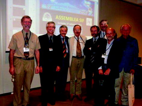
From left to right, Peter Wagner, Fabio Benfenati (then President of the Italian Physiological Society), Arsenio Veicsteinas, Pietro Enrico di Prampero, Guido Ferretti, Fabio Esposito, Carlo Capelli and Paolo Cerretelli. Wagner and di Prampero are the creators of the two multifactorial models of $\dot{V}\,{\text{O}}_{{2{ \max }}}$ limitation. Picture taken at the 62° annual meeting of the Italian Physiological Society, which took place in Sorrento, Italy, on 25–27 September 2011. Courtesy of Arsenio Veicsteinas

An Analysis of di Prampero’s Model

di Prampero’s model (di Prampero 1985, 2003; di Prampero and Ferretti 1990; Ferretti and di Prampero 1995) looks at the respiratory system from ambient air to the mitochondria as a hydraulic model of in-series resistances and assumes steady-state condition at maximal exercise. If this is so, for a system characterized by n resistances in series, we have:

$\dot{V} = \frac{{\Delta P_{1} }}{{R_{1} }} = \frac{{\Delta P_{2} }}{{R_{2} }} = \cdots = \frac{{\Delta P_{n} }}{{R_{n} }} = \frac{{\Delta P_{\text{T}} }}{{R_{\text{T}} }}$

(4.1)

where $\dot{V}$ is the gas flow, ΔP is the pressure gradient sustaining $\dot{V}$ across the ith resistance R and $\Delta P_{\text{T}}$ is the overall pressure gradient. At maximal exercise, $\dot{V}$ is $\dot{V}\,{\text{O}}_{{2{ \max }}}$ and $\Delta P_{\text{T}}$ is the difference between the inspired and the mitochondrial partial pressure of oxygen, $P_{I} {\text{O}}_{2} - P_{m} {\text{O}}_{2}$ . Since $P_{m} {\text{O}}_{2}$ tends to 0 mmHg (Gayeski and Honig 1986; Richardson et al. 2001; Wagner 2012), $\Delta P_{\text{T}}$ can be set equal to $P_{I} {\text{O}}_{2}$ with negligible error. Of course, ΔP_T is the sum of the pressure gradients across each resistance:

$\Delta P_{T} =\Delta P_{1} +\Delta P_{2} + \cdots +\Delta P_{n}$

(4.2)

In this case, the fraction of the overall limitation imposed by the ith resistance to oxygen flow is given by:

$F_{i} = \frac{{R_{i} }}{{R_{\text{T}} }}$

(4.3)

whence

$\frac{{R_{1} }}{{R_{\text{T}} }} + \frac{{R_{2} }}{{R_{\text{T}} }} + \cdots + \frac{{R_{n} }}{{R_{\text{T}} }} = F_{1} + F_{2} + \cdots + F_{n} = 1$

(4.4)

indicating that the overall limitation to oxygen flow in this model is equal to the sum of the fractional limitations imposed by each of the resistances in the system.

The portrait of the oxygen cascade presented in Fig. 1.3 allows identification of five resistances of clear physiological meaning, namely from proximal (ambient air) to distal (mitochondria), (i) the ventilatory resistance ( $R_{\text{V}}$ ), (ii) the lung resistance ( $R_{\text{L}}$ ), which refers to the transfer of oxygen from the alveoli to the arterial blood, (iii) the cardiovascular resistance ( $R_{\text{Q}}$ ), (iv) the tissue resistance ( $R_{\text{t}}$ ), which refers to oxygen transfer from peripheral capillaries to muscle fibres and (v) the mitochondrial resistance ( $R_{\text{m}}$ ), related to mitochondrial oxygen flow and utilization. Although these resistances are related to general concepts that can easily be perceived, discrimination between $R_{\text{t}}$ and $R_{\text{m}}$ is virtually impossible, because they are strongly interrelated on a structural basis. Therefore, for subsequent analysis, they are merged to form a lumped peripheral resistance ( $R_{\text{p}}$ ). For the specific case of $\dot{V}\,{\text{O}}_{{2{ \max }}}$ , Eq. (4.1) can thus be rewritten as follows:

$\dot{V}\,{\text{O}}_{{2{ \max }}} = \frac{{(P_{I} {\text{O}}_{2} - P_{A} {\text{O}}_{2} )}}{{R_{\text{V}} }} = \frac{{(P_{A} {\text{O}}_{2} - P_{a} {\text{O}}_{2} )}}{{R_{\text{L}} }} = \frac{{(P_{a} {\text{O}}_{2} - P_{{\bar{v}}} {\text{O}}_{2} )}}{{R_{\text{Q}} }} = \frac{{P_{{\bar{v}}} {\text{O}}_{2} }}{{R_{\text{p}} }} = \frac{{P_{I} {\text{O}}_{2} }}{{R_{\text{T}} }}$

(4.5)

Of these resistances, only two are characterized by precisely defined physiological variables, namely $R_{\text{V}}$ and $R_{\text{Q}}$ , which are, respectively, equal to:

$R_{V} = \frac{1}{{\dot{V}_{\text{A}} \cdot \beta_{g} }}$

(4.6a)

$R_{\text{Q}} = \frac{1}{{\dot{Q} \cdot \beta_{b} }}$

(4.6b)

where $\dot{V}_{A}$ is alveolar ventilation and $\dot{Q}$ is cardiac output. The other two variables are the oxygen transfer coefficient for air ( $\beta_{g}$ ) and for blood ( $\beta_{b}$ ), i.e. the volume of oxygen that can be displaced across a gradient of a unit of pressure. In STPD condition, $\beta_{g}$ is equal to 1.16 ml mmHg⁻¹ and is an invariant constant. Concerning $\beta_{b}$ , it is equal to:

$\beta_{b} = \frac{{(Ca{\text{O}}_{2} - C\bar{v}{\text{O}}_{2} )}}{{(Pa{\text{O}}_{2} - P\bar{v}{\text{O}}_{2} )}}$

(4.7)

that is the average slope of the oxygen equilibrium curve. Therefore, constant $\beta_{b}$ is not an invariant value, for it depends on the oxygen pressure range on which blood operates. The other three resistances cannot be translated into equivalent physiological expressions. $R_{\text{L}}$ , $R_{\text{t}}$ and $R_{\text{m}}$ were set proportional, respectively, to a factor including lung diffusing capacity corrected for the effect of $\dot{V}_{A} /\dot{Q}$ heterogeneity, to muscle capillary density and to muscle mitochondrial volume (di Prampero and Ferretti 1990).

When a manipulation, either chronic or acute, affects $\dot{V}\,{\text{O}}_{{2{ \max }}}$ without affecting $P_{I} {\text{O}}_{2}$ , and thus ΔP _T, the observed increase in $\dot{V}\,{\text{O}}_{{2{ \max }}}$ is the result of changes in one or more of the resistances in series. Thus, the model was devised in such a manner as to provide a value for the fraction of the overall $\dot{V}\,{\text{O}}_{{2{ \max }}}$ limitation which any given in-series resistance is responsible for. For instance, aerobic training provides a given $\dot{V}\,{\text{O}}_{{2{ \max }}}$ increase, $\Delta \dot{V}\,{\text{O}}_{{2{ \max }}}$ , because some resistances (at least three in this case, namely $R_{\text{Q}}$ , $R_{\text{t}}$ and $R_{\text{m}}$ ) have decreased, and so has $R_{\text{T}}$ . Thus, after training has induced a measurable increase in $\dot{V}\,{\text{O}}_{{2{ \max }}}$ with respect to the value before training, Eq. (4.5) can be rewritten as follows:

$\dot{V}\,{\text{O}}_{{2{ \max }}} +\Delta \dot{V}\,{\text{O}}_{{2{ \max }}} = \frac{{P_{I} {\text{O}}_{2} }}{{(R_{\text{T}} +\Delta R_{\text{T}} )}}$

(4.8)

If we divide Eq. (4.5) by Eq. (4.8), we get:

$\frac{{\dot{V}\,{\text{O}}_{{2{ \max }}} }}{{\left(\dot{V}\,{\text{O}}_{{2{ \max }}} +\Delta \dot{V}\,{\text{O}}_{{2{ \max }}} \right)}} = 1 + \frac{{\Delta R_{\text{T}} }}{{R_{\text{T}} }}$

(4.9)

which, since $\Delta R_{\text{T}}$ is the sum of the changes in the ith resistances in series, it can also take the following form:

$\frac{{\dot{V}\,{\text{O}}_{{2{ \max }}} }}{{(\dot{V}\,{\text{O}}_{{2{ \max }}} +\Delta \dot{V}\,{\text{O}}_{{2{ \max }}} )}} = 1 + \frac{{(\Delta R_{\text{V}} +\Delta R_{\text{L}} +\Delta R_{\text{Q}} +\Delta R{\text{p}}) }}{{R_{\text{T}} }}$

(4.10)

As a consequence of Eqs. (4.3) and (4.4), the induction of a change in any resistance by a manoeuvre specifically acting on it yields:

$\frac{{\Delta R_{i} }}{{R_{\text{T}} }} = F_{i} \cdot \frac{{\Delta R_{i} }}{{R_{i} }}$

(4.11)

So, Eq. (4.10) can be rewritten as follows:

$\frac{{\dot{V}\,{\text{O}}_{{2{ \max }}} }}{{\left( {\dot{V}\,{\text{O}}_{{2{ \max }}} +\Delta \dot{V}\,{\text{O}}_{{2{ \max }}} } \right)}} = 1 + F_{\text{V}} \frac{{\Delta R_{\text{V}} }}{{R_{\text{V}} }} + F_{\text{L}} \frac{{\Delta R_{\text{L}} }}{{R_{\text{L}} }} + F_{\text{Q}} \frac{{\Delta R_{\text{Q}} }}{{R_{\text{Q}} }} + F_{\text{p}} \frac{{\Delta R_{\text{p}} }}{{R_{\text{p}} }}$

(4.12)

Equation (4.12) has four unknowns and as such cannot be solved. However, if we take a condition wherein only one resistance is varied by an acute manipulation, as is the case, according to di Prampero and Ferretti (1990), for $R_{\text{Q}}$ after acute blood reinfusion or withdrawal, three terms of Eq. (4.12) annihilate. Thus, we remain with a simplified version of it, with only one unknown. For the specific case of changes in $R_{\text{Q}}$ only, Eq. (4.12) takes therefore the following form:

$\frac{{\dot{V}\,{\text{O}}_{{2{ \max }}} }}{{\left( {\dot{V}\,{\text{O}}_{{2{ \max }}} +\Delta \dot{V}\,{\text{O}}_{{2{ \max }}} } \right)}} = 1 + F_{\text{Q}} \frac{{\Delta R_{\text{Q}} }}{{R_{\text{Q}} }}$

(4.13)

Equation (4.13) allows computation of $F_{\text{Q}}$ , provided we know the $\dot{V}\,{\text{O}}_{{2{ \max }}}$ before and after the manoeuvre, the $R_{\text{Q}}$ before the manoeuvre and the absolute change in $R_{\text{Q}}$ induced by the manoeuvre. An analytical solution of Eq. (4.13), using data from different sources in the literature, is reported in Fig. 4.3, where the ratio between the $\dot{V}\,{\text{O}}_{{2{ \max }}}$ values before and after the manoeuvre (left-hand branch of Eq. 4.13) is plotted as a function of the ratio between $\Delta R_{\text{Q}}$ and $R_{\text{Q}}$ . Equation (4.13) tells that this relationship is linear, with y-intercept equal to 1 and slope equal to $F_{\text{Q}}$ . From linear regression analysis of the data shown in Fig. 4.3, di Prampero and Ferretti (1990) obtained $F_{\text{Q}} = 0.70$ . This means that $R_{\text{Q}}$ provides 70 % of the fractional limitation of $\dot{V}\,{\text{O}}_{{2{ \max }}}.$

An $F_{\text{Q}}$ value equal to 0.70 implies that the respiratory system does not have linear behaviour. In fact, for a linear respiratory system, the ratio of any given $R_{i}$ to $R_{\text{T}}$ would be equal to the ratio of the pressure gradient over that $R_{i}$ to the overall pressure gradient, so that:

$F_{\text{Q}} = \frac{{(Pa{\text{O}}_{2} - P\bar{v}{\text{O}}_{2} )}}{{P_{I} {\text{O}}_{2} }}$

(4.14)

from which we would have obtained $F_{\text{Q}} = 0.50$ instead of 0.70 (di Prampero and Ferretti 1990). The source of nonlinearity, and thus the source of this discrepancy, was identified in the effects of the oxygen equilibrium curve on $\beta_{b}$ , as shown in Fig. 4.4. Assume that an acute manoeuvre acts directly on $R_{\text{V}}$ only, e.g. reducing it. This would increase $P_{A} {\text{O}}_{2}$ , and thus $Pa{\text{O}}_{2}$ , but would not change the associated $Ca{\text{O}}_{2}$ , because in normoxia our blood operates on the flat portion of the oxygen equilibrium curve. Therefore, since $P\bar{v}{\text{O}}_{2}$ undergoes only small changes, $\beta_{b}$ would be reduced, and thus $R_{\text{Q}}$ would be increased. In sum, because of the shape of the oxygen equilibrium curve, as long as we are in normoxia, a specific manoeuvre acting only on $R_{\text{V}}$ cannot have effects on $\dot{V}\,{\text{O}}_{{2{ \max }}}$ , because any change in $R_{\text{V}}$ would be counteracted by an opposite change in $R_{\text{Q}}$ : in normoxia, $\varvec{R}_{{\mathbf{V}}}$ and $\varvec{R}_{{\mathbf{L}}}$ do not limit ${\varvec{\dot{V}}}\,{\mathbf{O}}_{{{\mathbf{2max}}}}$ . Using a different terminology, this is the case when perfusion limitation characterises the alveolar-capillary gas transfer. Thus, the effects of the respiratory system on $\dot{V}\,{\text{O}}_{{2{ \max }}}$ can be fully described by a two-site model wherein the effective limitation is located distally to $Pa{\text{O}}_{2}$ . This explains why $F_{\text{Q}} = 0.7$ instead of 0.5, so that we necessarily have $F_{\text{p}} = 0.3$ , partly attributable to $F_{\text{t}}$ , partly to $F_{\text{m}}$ . According to Ferretti et al. (1997a), the differences in $\dot{V}\,{\text{O}}_{{2{ \max }}}$ would be minimal, if we assume, on one extreme, $R_{\text{t}} = R_{\text{p}}$ , and on the other extreme, $R_{\text{m}}$ = $R_{\text{p}}$ , and that it makes no difference to assume $R_{\text{t}}$ and $R_{\text{m}}$ in series or in parallel. Direct experimental assessment of the parameters of Eq. (4.13) confirmed that $F_{\text{Q}}$ in normoxia is between 0.65 and 0.76 (Bringard et al. 2010; Turner et al. 1993).

Fig. 4.3

Graphical representation of Eq. (4.13). The changes in $\dot{V}\,{\text{O}}_{{2{ \max }}}$ that follow an acute manoeuvre acting on the cardiovascular resistance to oxygen flow (Rq) are expressed as the ratio of the $\dot{V}\,{\text{O}}_{{2{ \max }}}$ before to the $\dot{V}\,{\text{O}}_{{2{ \max }}}$ after the manoeuvre at stake ( $\dot{V}\,{\text{O}}_{{2{ \max }}} +\Delta$ ). This ratio is plotted as a function of the ratio between the induced change in $R_{\text{Q}}$ ( $\Delta R_{\text{Q}}$ ) and the $R_{\text{Q}}$ before the manoeuvre. Points are mean values from different sources in the literature. The continuous straight line is the corresponding regression equation (y = 1.006 + 0.7 x, r = 0.97, n = 15). The slope of the line, equal to 0.7, indicates that 70 % of the overall limitation to $\dot{V}\,{\text{O}}_{{2{ \max }}}$ is imposed by cardiovascular oxygen transport. Modified after di Prampero and Ferretti (1990)

Fig. 4.4

Average oxygen equilibrium curve. Two arterial and mixed venous points are reported, applying to normaemia ( $a_{0}$ , $\bar{v}_{0}$ ) and hypoxaemia ( $a_{1}$ , $\bar{v}_{1}$ ). The two straight lines connecting the two couples of points have a slope equal to the respective oxygen transport coefficients for blood ( $\beta_{b}$ ), which is higher in hypoxaemia than in normaemia. As a consequence, when an increase in the ventilatory resistance $R_{\text{V}}$ entails a decrease in arterial oxygen partial pressure, $\beta_{b}$ becomes higher and the cardiovascular resistance $R_{\text{Q}}$ lower. These two phenomena compensate each other, so that no changes in $\dot{V}\,{\text{O}}_{{2{ \max }}}$ are induced by an acute change in $R_{\text{V}}$ : the lungs do not limit $\dot{V}\,{\text{O}}_{{2{ \max }}}$ in normoxia. Modified after di Prampero (1985)

Experimental Testing of di Prampero’s Model

The nonlinear behaviour of the respiratory system implies that within the context of di Prampero’s model (i) $R_{\text{V}}$ and $R_{\text{L}}$ do limit $\dot{V}\,{\text{O}}_{{2{ \max }}}$ in hypoxia; (ii) $F_{\text{Q}}$ in hypoxia is less than 0.7; (iii) the decrease of $\dot{V}\,{\text{O}}_{{2{ \max }}}$ in hypoxia is larger in subjects with high $\dot{V}\,{\text{O}}_{{2{ \max }}}$ in normoxia; (iv) only subjects with high $\dot{V}\,{\text{O}}_{{2{ \max }}}$ in normoxia undergo an increase in $\dot{V}\,{\text{O}}_{{2{ \max }}}$ in hyperoxia; (v) exercise with small muscle masses reduces $F_{\text{Q}}$ and increases $F_{\text{p}}$ ; (vi) the fall of $\dot{V}\,{\text{O}}_{{2{ \max }}}$ in hypoxia is smaller, the smaller is the contracting muscle mass. Moreover, since the cause of the nonlinear behaviour of the respiratory system is related to the shape of the oxygen equilibrium curve, there must be a linear relationship between $\dot{V}\,{\text{O}}_{{2{ \max }}}$ and SaO₂.

To investigate the roles played by $R_{\text{V}}$ and $R_{\text{L}}$ in normoxia and hypoxia, Esposito and Ferretti (1997) changed the air density of the inspired gas mixture by replacing nitrogen with helium, thus reducing $R_{\text{V}}$ . Although $\dot{V}_{A}$ increased in both cases, $\dot{V}\,{\text{O}}_{{2{ \max }}}$ did not change when breathing the He–O₂ mixture in normoxia, going up only in hypoxia. Similar results were recently obtained also by Ogawa et al. (2010). Consistently, no effects of respiratory muscle training were shown on $\dot{V}\,{\text{O}}_{{2{ \max }}}$ in normoxia, but a positive effect was observed in hypoxia (Downey et al. 2007; Esposito et al. 2010).

On two groups of subjects, one with high, the other with low $\dot{V}\,{\text{O}}_{{2{ \max }}}$ in normoxia, Ferretti et al. (1997b) found that, in the former with respect to the latter group, (i) the decrease in $\dot{V}\,{\text{O}}_{{2{ \max }}}$ in hypoxia was larger, and (ii) a significant increase in $\dot{V}\,{\text{O}}_{{2{ \max }}}$ in hyperoxia occurred. Moreover, they found a highly significant linear relationship between $\dot{V}\,{\text{O}}_{{2{ \max }}}$ , expressed relative to the value in hyperoxia set equal to 100 %, and SaO₂, which was identical in both groups, in agreement with the above predictions. According to Wehrlin and Hallén (2006), the $\dot{V}\,{\text{O}}_{{2{ \max }}}$ of endurance athletes is so high that the decrease of $\dot{V}\,{\text{O}}_{{2{ \max }}}$ in hypoxia becomes linear. Coherent with this picture is also the finding that the $\dot{V}\,{\text{O}}_{{2{ \max }}}$ decrease in hypoxia is smaller the stronger is the ventilatory response to hypoxia (Benoit et al. 1995; Gavin et al. 1998; Kayser et al. 1994; Marconi et al. 2004).

An Analysis of Wagner’s Model

Peter Wagner (1993) constructed a three-equation system with three unknowns ( $P_{A} {\text{O}}_{2}$ , $P_{a} {\text{O}}_{2}$ and $P_{{\bar{v}}} {\text{O}}_{2}$ ) by combining the mass conservation equation for blood (Fick principle) and the two diffusion–perfusion interaction equations (Piiper and Scheid 1981; Piiper et al. 1984). At steady state, all these equations must have equal solutions for $\dot{V}\,{\text{O}}_{{2{ \max }}}$ . The algebraic development of the system led to three equations allowing a solution for $P_{A} {\text{O}}_{2}$ , $P_{a} {\text{O}}_{2}$ and $P_{{\bar{v}}} {\text{O}}_{2}$ . These equations lead to a unique, necessary $\dot{V}\,{\text{O}}_{{2{ \max }}}$ value for any combination of known values of $P_{I} {\text{O}}_{2}$ , $\dot{V}_{A}$ , D _L, $\dot{Q}$ , $\beta_{b}$ and D _t at maximal exercise (Wagner 1993). Wagner’s system of equations implies a vision of the oxygen cascade with two mass balance equations responsible for convective oxygen transfer, associated with two conductive components, described by the diffusion–perfusion interaction equations. This vision is conceptually different from di Prampero’s, who conceived a pure hydraulic system of in-series resistances. Proximally, the interaction of a convective component with a diffusive component sets the maximal flow of oxygen in arterial blood ( $\dot{Q}a{\text{O}}_{{2{ \max }}}$ ), and this is the first step in the system. Distally, the interaction of a convective component (Fick principle) with a diffusive component (the diffusion–perfusion interaction equation setting oxygen flow from peripheral capillaries to the muscle fibres) sets $\dot{V}\,{\text{O}}_{{2{ \max }}}$ .

The Fick equation can take either of the following solutions:

$\dot{V}\,{\text{O}}_{{2{ \max }}} = \dot{Q} \cdot \left( {Ca{\text{O}}_{2} - C\bar{v}{\text{O}}_{2} } \right) = \dot{Q} \cdot \beta_{b} \cdot \left( {P_{a} {\text{O}}_{2} - P_{{\bar{v}}} {\text{O}}_{2} } \right)$

(4.15)

The term $\beta_{b}$ in Eq. (4.15) implies a nonlinear negative relationship between $\dot{V}\,{\text{O}}_{{2{ \max }}}$ and $P_{{\bar{v}}} {\text{O}}_{2}$ (convective curve), the algebraic expression of which depends on the solution that is given to the oxygen equilibrium curve. Concerning the diffusive component, it is described by the following equation:

$\dot{V}\,{\text{O}}_{{2{ \max }}} = D{\text{tO}}_{2} \cdot \left( {P_{{\bar{c}}} {\text{O}}_{2} - P_{m} {\text{O}}_{2} } \right)$

(4.16)

where $D{\text{tO}}_{2}$ is tissue diffusing capacity for oxygen and $P_{m} {\text{O}}_{2}$ is again equal to 0 mmHg. However, the right branches of Eqs. (4.15) and (4.16) do not share any term, so that they cannot as such be compared on the same plot. To circumvent this obstacle, Wagner assumed direct proportionality between $P_{{\bar{v}}} {\text{O}}_{2}$ and $P_{{\bar{c}}} {\text{O}}_{2}$ , arguing that the segment of the oxygen equilibrium curve between these two pressure values is essentially linear, so that within that segment $\beta_{b}$ can be considered invariant. On this basis, he reformulated Eq. (4.16) as follows:

$\dot{V}\,{\text{O}}_{{2{ \max }}} = D{\text{tO}}_{2} \cdot K_{\text{p}} \cdot P_{{\bar{v}}} {\text{O}}_{2}$

(4.17)

where $K_{\text{p}}$ is the dimensionless constant relating $P_{{\bar{v}}} {\text{O}}_{2}$ and $P_{{\bar{c}}} {\text{O}}_{2}$ . Equation (4.17) implies a positive linear relationship between $\dot{V}\,{\text{O}}_{{2{ \max }}}$ and $P_{{\bar{v}}} {\text{O}}_{2}$ (diffusion line), which Roca et al. (1989) determined experimentally. The slope of the line is equal to the product $D{\text{tO}}_{2} \cdot K_{\text{p}}$ , which Ferretti (2014) called Wagner’s constant, $K_{\text{W}}$ . Equations (4.15) and (4.17) generate analytical relationships that, if we plot $\dot{V}\,{\text{O}}_{{2{ \max }}}$ on the y-axis and $P_{{\bar{v}}} {\text{O}}_{2}$ on the x-axis, can be represented on the same graph and directly compared (Fig. 4.5). In this figure, the resulting $\dot{V}\,{\text{O}}_{{2{ \max }}}$ for any combination of $\dot{Q}a{\text{O}}_{{2{ \max }}}$ and $K_{\text{W}}$ corresponds to the intersection of the two functions, which occurs at a precise value of $P_{{\bar{v}}} {\text{O}}_{2}$ .

Fig. 4.5

Graphical representation of Wagner’s model. Oxygen uptake ( $\dot{V}\,{\text{O}}_{2}$ ) is plotted as a function of mixed venous oxygen pressure ( $P_{{\bar{v}}} {\text{O}}_{2}$ ). The curve with negative slope is Wagner’s convective curve. The straight line with positive slope is Wagner’s diffusion line, whose slope is equal to Wagner’s constant $K_{\text{W}}$ . The convective curve intercepts the y-axis at a $\dot{V}\,{\text{O}}_{2}$ equal to arterial oxygen flow ( $\dot{Q}a{\text{O}}_{2}$ ), which is the case when $K_{\text{W}}$ = ∞. The same curve intercepts the x-axis when $P_{{\bar{v}}} {\text{O}}_{2}$ is equal to arterial oxygen pressure, which is the case when $K_{\text{W}}$ = 0. The $\dot{V}\,{\text{O}}_{{2{ \max }}}$ value is found on the crossing of the convective curve with the diffusion line (full dot). After Ferretti (2014)

Experimental Testing of Wagner’s Model

Concerning the diffusive component, a decrease in $D{\text{tO}}_{2}$ implies, in Fig. 4.5, a decrease in $K_{\text{W}}$ , whence a drop of $\dot{V}\,{\text{O}}_{{2{ \max }}}$ and an increase in $P_{{\bar{v}}} {\text{O}}_{2}$ . The reverse is caused by an increase in $D{\text{tO}}_{2}$ . This is virtually impossible to test in humans with acute manoeuvres acting on $D{\text{tO}}_{2}$ , the most important determinant of $K_{\text{W}}$ . Moreover, $D{\text{tO}}_{2}$ is affected by haemoglobin concentration (Schaffartzik et al. 1993). Wagner (1996a) predicted quite accurately the effects of chronic alterations of $D{\text{tO}}_{2}$ on $\dot{V}\,{\text{O}}_{{2{ \max }}}$ and $P_{{\bar{v}}} {\text{O}}_{2}$ in patients affected by chronic obstructive pulmonary disease, once allowance was made for the simultaneous impairment of cardiovascular oxygen transport. If direct proportionality between $K_{\text{W}}$ and muscle capillary density is assumed, an analysis of literature data of muscle morphometry and $\dot{V}\,{\text{O}}_{{2{ \max }}}$ of altitude-acclimatized climbers (Hoppeler et al. 1990; Oelz et al. 1986) or endurance-trained subjects (Hoppeler et al. 1985) led to $P_{{\bar{v}}} {\text{O}}_{2}$ values coherent with Wagner’s predictions (Ferretti 2014).

On the convective curve, an increase in the product of $\dot{Q}$ times $\beta_{b}$ carries along an increase in both $\dot{V}\,{\text{O}}_{{2{ \max }}}$ and $P_{{\bar{v}}} {\text{O}}_{2}$ . This explains, in Wagner’s model, the effects of acute polycythaemia and anaemia on $\dot{V}\,{\text{O}}_{{2{ \max }}}$ (Ekblom et al. 1976; Woodson et al. 1978): the convective curve is displaced upwards and becomes steeper. The intercept on the x-axis of the convective curve corresponds to the $P_{a} {\text{O}}_{2}$ point, i.e. the point at which $P_{{\bar{v}}} {\text{O}}_{2} = P_{a} {\text{O}}_{2}$ . Hyperoxia displaces this point to the right, implying a slightly higher $\dot{V}\,{\text{O}}_{{2{ \max }}}$ , because the rightward displacement of the $P_{a} {\text{O}}_{2}$ point increases the slope of the convective curve (makes it less negative), so that the diffusion line is intercepted at a higher $\dot{V}{\text{O}}_{{2{ \max }}}$ value. The reverse occurs in hypoxia. The y-intercept of the convective curve corresponds to the $\dot{Q}a{\text{O}}_{{2{ \max }}}$ point, representing the condition in which $\dot{V}\,{\text{O}}_{{2{ \max }}} = \dot{Q}a{\text{O}}_{{2{ \max }}}$ (Wagner 1995, 1996a). The case of hypoxia is treated in a separate paragraph (see Of Maximal Oxygen Consumption in Hypoxia). Controversial is the case of hyperoxia. Although Fig. 4.5 predicts an increase in $\dot{V}\,{\text{O}}_{{2{ \max }}}$ , such an increase was rarely observed in humans, the only clear effects having been observed in individuals with elevated $\dot{V}\,{\text{O}}_{{2{ \max }}}$ , who are subject to the Dempsey effect (Dempsey and Wagner 1999; Dempsey et al. 1984; Powers et al. 1989). Richardson et al. (1999) were able to observe a $\dot{V}\,{\text{O}}_{{2{ \max }}}$ increase during single-leg exercise only when they used pure oxygen breathing. The thoroughbred horse, a highly athletic animal characterized by deep hypoxaemia at maximal exercise, was proposed as the nicest example supporting the prediction of elevated $\dot{V}\,{\text{O}}_{{2{ \max }}}$ in hyperoxia (Wagner 1996a; Wagner et al. 1989, 1996). This apparent discrepancy between theoretical predictions and experimental data is hard to explain, and the hypotheses put forward so far are scarcely convincing, so that the issue still remains open.

Only gold members can continue reading. Log In or Register to continue