Kinematic and Computational Model of Human Ankle

(7.2) is the homogeneous transformation matrix, $R_{AB} \in {{\mathbb{R}}}^{3 \times 3}$ is the orthonormal matrix that describes the orientation of frame B with respect to frame A and $t_{AB} \in {{\mathbb{R}}}^{3}$ is the translation from origin of frame A to frame B (expressed in frame A). $x_{A} \in {{\mathbb{R}}}^{3}$ is the location of the point relative to the origin of frame A, expressed in frame A coordinates. Similarly, $x_{B} \in {{\mathbb{R}}}^{3}$ is the location of the point relative to the origin of frame B, expressed in frame B coordinates. A diagram depicting these is shown in Fig. 7.1. It is also useful to note that the inverse of a homogeneous transformation matrix can be represented by (4.3).

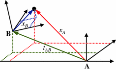
Fig. 7.1

Graphical representation of variables used

$\left[ {\begin{array}{*{20}c} {x_{A} } \\ 1 \\ \end{array} } \right] = T_{AB} \left[ {\begin{array}{*{20}c} {x_{B} } \\ 1 \\ \end{array} } \right]$

(7.1)

${T_{AB}}^{ - 1} = T_{BA} = \left[ {\begin{array}{*{20}c} {{R_{AB}}^{\text{T}} } & {{ - R_{AB}}^{\text{T}} t_{AB} } \\ {0_{1 \times 3} } & 1 \\ \end{array} } \right]$

(7.2)

Using the homogeneous transformation matrices, the ankle, subtalar and foot coordinate frames can be defined with respect to a fixed global frame. These frames are shown in Fig. 7.2. For the purpose of this research, all foot bones from the calcaneus to the phalanges were considered as one single rigid body and its orientation and translation were represented by the foot coordinate frame. The subtalar frame was taken to be located on the talus, where its position is fixed and its orientation can change via rotation about the subtalar joint (red axis in the subtalar frame). Similarly, the ankle frame was considered to be fixed on the tibia in terms of location and free to rotate about the ankle joint axis (red axis of the ankle frame). Since the axes of revolution are denoted as the x-axes of the coordinate frames, the orientation of the ankle frame with respect to the global coordinates can be represented by consecutively applying rotations about the y- and z-axes of the global frame, while the subtalar frame can be obtained by applying y- and z-rotations about the ankle frame. Each of these frames also uses three translations to reposition its origin at designated points in the global frame. A total of five parameters were therefore required to define each of the ankle and subtalar frames at the foot’s neutral position. For convenience, the orientation of the foot coordinate frame was taken to be identical to that of the global frame and three parameters were used to determine the origin of the foot frame.

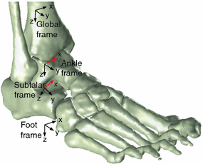
Fig. 7.2

The superposition of indicative ankle, subtalar, foot and global coordinate frames on a three-dimensional surface model of the foot–ankle structure. Red axes represent the axes about which rotations occur

The homogeneous transformation matrices representing the ankle, subtalar and foot coordinate frames at the neutral foot position are given by (7.3)–(7.5), where $R_{z}$ and $R_{y}$ are, respectively, the rotational transformation matrices about the z- and y-axes, and subscripts

and f are used to represent quantities related to the ankle, subtalar and foot coordinate frames. It should also be noted that subscript i is used to indicate a variable’s correspondence to the neutral foot position.

$T_{0a,i} = \left[ {\begin{array}{*{20}c} {R_{0a,i} } & {t_{0a} } \\ {0_{1 \times 3} } & 1 \\ \end{array} } \right] = \left[ {\begin{array}{*{20}c} {R_{z,a} R_{y,a} } & {t_{0a} } \\ {0_{1 \times 3} } & 1 \\ \end{array} } \right]$

(7.3)

$T_{0s,i} = T_{0a,i} T_{as,i} = T_{0a,i} \left[ {\begin{array}{*{20}c} {R_{as,i} } & {t_{as,i} } \\ {0_{1 \times 3} } & 1 \\ \end{array} } \right] = T_{0a,i} \left[ {\begin{array}{*{20}c} {R_{z,s} R_{y,s} } & {t_{as,i} } \\ {0_{1 \times 3} } & 1 \\ \end{array} } \right]$

(7.4)

$T_{0f,i} = \left[ {\begin{array}{*{20}c} {R_{0f,i} } & {t_{0a} } \\ {0_{1 \times 3} } & 1 \\ \end{array} } \right] = \left[ {\begin{array}{*{20}c} {I_{3} } & {t_{0f,i} } \\ {0_{1 \times 3} } & 1 \\ \end{array} } \right]$

(7.5)

Since x-axis rotations are permissible at the ankle and subtalar joints, the final homogeneous transformation matrix associated with the foot frame can be obtained by including the angular displacements at the ankle and subtalar joints as shown in (7.6), where $R_{x}$ is used to represent the transformation matrix for an x-axis rotation. It can be seen that the foot coordinate frame at the neutral position is recovered when both the ankle and subtalar displacements are zero.

$T_{0f} = T_{0a,i} \left[ {\begin{array}{*{20}c} {R_{x,a} } & {0_{3 \times 1} } \\ {0_{1 \times 3} } & 1 \\ \end{array} } \right]T_{0a,i}^{ - 1} T_{0s,i} \left[ {\begin{array}{*{20}c} {R_{x,s} } & {0_{3 \times 1} } \\ {0_{1 \times 3} } & 1 \\ \end{array} } \right]T_{0s,i}^{ - 1} T_{0f,i}$

(7.6)

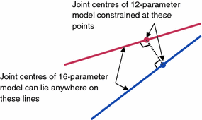
It is worth noting that the model formulated above will generally have 16 parameters. This is because six parameters will be required to define $T_{0f,i}$ if the orientation of the neutral foot frame is left arbitrary. As the models proposed by van den Bogert et al. [1] and Lewis et al. [2] only use 12 parameters, the model presented above is not a minimal realisation of the biaxial model. Two of the four additional parameters can be viewed as the angular offsets needed at each revolute joint to zero the ankle and subtalar joint displacements at the neutral foot orientation. The presence of the remaining two parameters is related to the fact that the origins for the ankle and subtalar frame can be placed anywhere along the corresponding revolute axis (as illustrated in Fig. 7.3). This means an additional degree of freedom is used for the location of each of these origins. While the 16-parameter model allows arbitrary combinations of origins along these two axes, the location of these origins is constrained in the 12-parameter model to lie on points where the distance between lines representing the two axes is at its minimum. For the purpose of simulation, the added number of parameters will not make any difference to the resulting foot motion as these models describe identical kinematic constraints.

Fig. 7.3

Diagram showing additional degrees of freedom available in the 16-parameter kinematic model when compared with the 12-parameter model

7.1.1 Identification of the Reduced Biaxial Model

Where parameter identification is concerned, additional parameters will introduce redundancy in the system to be identified and this may lead to problems in estimation results. Models with no redundancy are therefore preferred in the formulation of system identification problems. However, while algorithms used in [1, 2] are designed to identify both orientation and location of the ankle and subtalar revolute joints, the emphasis of the identification algorithm in this research is mainly on the orientations of the ankle and subtalar joint axes, which are required for controller parameter adaptation strategies, the translations of the foot rigid bodies are therefore not considered in the proposed parameter identification scheme and the redundant parameters used to describe the joint centres in the kinematic formulation presented above were not of any interest in this work. It is also important in this application that the neutral foot position corresponds with zero ankle and subtalar joint displacements, and it can be seen that this condition is inherently satisfied in the kinematic model defined above, hence justifying the inclusion of the two additional axis orientation parameters in the proposed estimation problem.

The foot orientation as obtained from the kinematic model, $\widehat{R}_{0f}$ , is represented by the rotational transformation matrix and it takes the form of (7.7) when the initial orientation of the foot is taken to be identical to that of the global reference frame.

$\widehat{R}_{0f} = R_{0a,i} R_{x,a} R_{as,i} R_{x,s} {R_{as,i}}^{\text{T}} {R_{0a,i}}^{\text{T}}$

(7.7)

As previously discussed, $R_{0a,i}$ and $R_{0s,i}$ can each be defined using two rotations. A biaxial kinematic model with fixed revolute joints therefore has four parameters governing its final orientation. Since these are the only parameters of interest for this work, the identification problem used in this application can be made simpler than that described in [1, 2], thus making it more feasible for online implementation.

Formally, the kinematic model considered in this study is represented by (7.8). It can be seen that this model outputs the model foot orientations in terms of Euler angles $\widehat{\Theta }$ and uses the model parameters, $\rho$ , and joint displacements, $\theta_{as}$ , as inputs. Here, $\rho = \left[ {\begin{array}{*{20}c} {\theta_{z,a} } & {\theta_{y,a} } & {\theta_{z,s} } & {\theta_{y,s} } \\ \end{array} } \right]^{\text{T}}$ , where $\theta_{z,a}$ is the z-rotation angle for the ankle axis, $\theta_{y,a}$ is the y-rotation angle for the ankle axis, $\theta_{z,s}$ is the z-rotation angle for the subtalar axis, and $\theta_{y,s}$ is the y-rotation angle for the subtalar axis. These parameters will be collectively referred to as the axis tilt angles hereafter.

$\widehat{\Theta } = f\left( {\rho ,\theta_{as} } \right) = g\left( {\rho ,{\Theta}} \right)$

(7.8)

Since the ankle and subtalar joint angles cannot be readily measured, they have to be estimated from the Euler angles used to describe the observed foot orientation, $\Theta$ . By keeping this in mind, it can be seen that $\widehat{\Theta }$ is in fact a function of $\rho$ and $\Theta$ . The parameter identification problem in this study is therefore one which seeks to minimise the differences between Euler angles estimated from the kinematic model and those obtained via measurement of the foot orientation. The desired model parameters are therefore the solution to (7.9), where k is the observation number and N the total number of observations.

$\mathop {\arg \hbox{min} }\limits_{{\rho \in \mathbb{R}^{4} }} \sum\limits_{k = 1}^{k = N} {\left[ {\Theta _{k} - g\left( {\rho ,\Theta _{k} } \right)} \right]^{\text{T}} \left[ {\Theta _{k} - g\left( {\rho ,\Theta _{k} } \right)} \right]}$

(7.9)

7.1.2 Gradient Computation of the Kinematic Model

The parameter identification of the ankle kinematic model is basically an optimisation problem, and the ability to compute the parameter gradient of the model will facilitate this process by permitting the use of line search optimisation routines. Despite the model being nonlinear in parameter, knowledge of its parameter gradient will still make the system amenable to application of online parameter identification algorithms such as the Kalman filter, the RLS and the least mean squares. This section will therefore describe the procedures required to compute this parameter gradient.

It can be seen that the output of the model is given in terms of Euler angles, while the foot orientation is presented in the form of a rotational matrix. An appropriate Euler angle convention must therefore be used to describe this orientation matrix. In this chapter, the ZXY Euler angles are used since this is the convention in which the measured pitch(X) and roll(Y) measurements are supplied by the inclinometer used in the prototype ankle rehabilitation robot. As the yaw component is not readily available from the inclinometer, it is computed by considering the forward kinematics of the robot. For completeness, the relationship between a rotational matrix and its corresponding ZXY Euler angles is given in (7.10), where $R_{x}$ is the matrix describing rotation about the x-axis by $\theta_{x}$ , $C_{x}$ is short for $\cos \theta_{x}$ , and $S_{x}$ is short for $\sin \theta_{x}$ . This notation extends to the y- and z-axes, where they are, respectively, indicated by the y and z subscripts. By representing the ZXY Euler angles in a column vector, it can be expressed as (7.11) when the foot orientation is known.

$R_{0f} = R_{z} R_{x} R_{y} = \left[ {\begin{array}{*{20}c} {C_{z} C_{y} - S_{z} S_{x} S_{y} } & { - S_{z} C_{x} } & {C_{z} S_{y} + S_{z} S_{x} C_{y} } \\ {S_{z} C_{y} + C_{z} S_{x} S_{y} } & {C_{z} C_{x} } & {S_{z} S_{y} - C_{z} S_{x} C_{y} } \\ { - C_{x} S_{y} } & {S_{x} } & {C_{x} C_{y} } \\ \end{array} } \right]$

(7.10)

$\Theta = \left[ {\begin{array}{*{20}c} {\theta_{x} } \\ {\theta_{y} } \\ {\theta_{z} } \\ \end{array} } \right] = \left[ {\begin{array}{*{20}c} {\sin^{ - 1} R_{0f32} } & {\tan^{ - 1} \left( {\frac{{ - R_{0f31} }}{{R_{0f33} }}} \right)} & {\tan^{ - 1} \left( {\frac{{ - R_{0f12} }}{{R_{0f22} }}} \right)} \\ \end{array} } \right]^{\text{T}}$

(7.11)

It is also clear from the previous discussion that ankle and subtalar joint displacements are a function of $\rho$ and $\Theta$ (7.12). As a result, the parameter gradient of the ZXY Euler angles in the ankle kinematic model can be obtained by considering (7.13).

$\theta_{as} = h\left( {\rho ,\Theta } \right)$

(7.12)

$\frac{{\partial \widehat{\Theta }}}{\partial \rho } = \frac{{\partial f\left( {\rho ,\theta_{as} } \right)}}{\partial \rho } + \frac{{\partial f\left( {\rho ,\theta_{as} } \right)}}{{\partial \theta_{as} }}\frac{{\partial \theta_{as} }}{\partial \rho }$

(7.13)

7.2 Online Identification of a Biaxial Ankle Model

The main objective of this work on ankle kinematic parameter estimation is to extract information of the orientations of the ankle and subtalar joint axes, while the ankle rehabilitation robot is in operation. An online parameter identification algorithm is therefore crucial for the realisation of this goal. This section will discuss the application of different online parameter identification algorithms to the kinematic parameter estimation problem in this research.

7.2.1 Online Identification Algorithms

7.2.1.1 Extended Kalman Filter/Recursive Least Square

The extended Kalman filter (EKF) is an algorithm for state estimation of nonlinear dynamic systems. It predicts system states by considering the measured system outputs, a state space model of the system dynamics and covariance matrices related to the uncertainties found in the measurements and system model. Kalman filters can also be used to simultaneously estimate both states and parameters of a system [3]. This can generally be achieved by augmentation of the parameters of interest to the system state vector. In this particular application, the emphasis is on obtaining an estimate of the system’s kinematic parameters. The dynamic model of the ankle and foot motion is therefore not considered.

The algorithm involved in the EKF has the same form as that of a conventional Kalman filter except for the use of linearised state transition and observation matrices. It should be noted, however, that while the Kalman filter is an optimal state estimator, the EKF is not optimal due to the linearisation of the output function. In this problem, the state transition matrix is simply an identity matrix, while the observation matrix is given by the gradient matrix computed from (7.19). The process and measurement noise covariance matrices will control the extent to which the filter will modify the model parameters to fit the measured data. The algorithm of the EKF for this application is given in Table 7.1.

Table 7.1

The EKF algorithm

Prediction step

$\begin{aligned} \hat{\rho }_{k|k - 1} & = \hat{\rho }_{k - 1|k - 1} \\ P_{k|k - 1} & = P_{k - 1|k - 1} + Q_{k} \\ \end{aligned}$

Update step

$\begin{aligned} \widetilde{\Theta }_{k} & =\Theta _{k} - g\left( {\hat{\rho}_{k|k - 1} ,\Theta _{k} } \right) \\ \hat{\rho }_{k|k} & = \hat{\rho }_{k|k - 1} + P_{k|k - 1} H_{k}^{T} \left( {H_{k} P_{k|k - 1} H_{k}^{T} + R_{k} } \right)^{ - 1} \widetilde{\Theta }_{k} \\ P_{k|k} & = \left[ {I - P_{k|k - 1} H_{k}^{T} \left( {H_{k} P_{k|k - 1} H_{k}^{T} + R_{k} } \right)^{ - 1} H_{k} } \right]P_{k|k - 1} \\ \end{aligned}$

where $H_{k} = \frac{{\partial {\widehat{\Theta}}}}{\partial \rho }$ and $$ I $$

is an identity matrix

The RLS algorithm is another common approach for online identification of linear models and is related to the Kalman filter. The RLS adaptive filter works by “memorising” previous measurements in the form of a cross-correlation matrix and the current estimated parameters. The correlation matrix is then used together with the estimation error of the current iteration to further adjust the model parameters. Even though the RLS algorithm will not produce the optimal estimates for nonlinear systems, its simplicity has warranted an investigation into its effectiveness for this application. Since the RLS algorithm works with linear systems, the linearised ankle kinematic model shown in (7.14) has to be used. It can be seen that the model is linearised about the set of parameters denoted by $\rho_{\text{lin}}$ and the measured ZXY Euler angles given by $\Theta$ . H is the gradient of the nonlinear model about its linearisation point and is used to relate changes in Euler angles to changes to the model parameters, with $\begin{array}{*{20}c} {\Delta\Theta=\widehat{\Theta}-\widehat{\Theta}_{\text{lin}}}\\\end{array}$ , $\Delta \hat{\rho } = \hat{\rho } - \rho_{\text{lin}}$ and $\widehat{\Theta }_{\text{lin}} = g\left( {\rho_{\text{lin}} ,\Theta } \right).$

$\widehat{\Theta}\approx g\left( {\rho_{\text{lin}},\Theta}\right)+\left. {\frac{{\partial\widehat{\Theta}}}{\partial\rho}}\right|_{{\rho_{\text{lin}},\Theta}}\left( {\hat{\rho}-\rho_{\text{lin}}}\right)\Rightarrow\Delta\Theta\approx H\Delta\rho$

(7.14)

Using this linear model, the RLS algorithm is given by (7.15), where $\Delta \hat{\rho }$ is the deviation in model parameter needed to reduce estimation error, $\hat{\rho }$ is the estimated parameter, P is the inverse cross-correlation matrix, λ is a geometric forgetting factor where a value of 1 will lead to all historical data being considered, k is the iteration number, and I is an identity matrix.

$P_{k} = \frac{1}{\lambda }\left[ {P_{k - 1} - P_{k - 1} {H_{k}}^{\text{T}} \left( {\lambda I + H_{k} P_{k - 1} {H_{k}}^{\text{T}} } \right)^{ - 1} H_{k} P_{k - 1} } \right]$

(7.15)

$\rho_{k} = \rho_{{{\text{lin}},k}} +\Delta \hat{\rho }_{k}$

(7.16)

A comparison of the RLS and EKF algorithm reveals that they are equivalent if:

The process noise covariance, Q, in the EKF is zero and the measurement noise covariance, R, is an identity matrix.

The geometric forgetting factor in the RLS algorithm is unity.

The parameters about which the model is linearised are the same as their estimates obtained from the previous iteration ( $\rho_{{{\text{lin}},k}} = \hat{\rho }_{k - 1}$ ).

Estimate of the parameter deviation vector brought forward from the previous iteration is always zero $(\Delta{\hat{\rho}}_{k - 1} = {\mathbf{0}}).$

Condition 1 above implies that the RLS algorithm is essentially an EKF which assumes that the model is perfect while allowing large uncertainties in the measurements. A look at conditions 3 and 4 also suggests that recurrent update of $\rho_{\text{lin}}$ and persistent reset of $\Delta \hat{\rho }$ will align the behaviour of the RLS algorithm with that of the EKF. Since the estimated gradient will become less accurate as the parameters deviate further from $\rho_{\text{lin}}$ , this frequent update should be able to improve on the accuracy of the RLS algorithm.

7.2.1.2 Least Mean Square

In addition to the EKF, the parameters of the kinematic model can also be estimated through the use of the least mean square algorithm. This algorithm uses the idea of steepest descent for parameter identification and therefore also requires information on the parameter gradient of the kinematic model. However, it does not explicitly store the previous measurements in memory as with the case of EKF or RLS and is therefore more efficient in terms of memory usage. It is also less complex as computation of the inverse cross-correlation matrix is not required.

The overall concept of this iterative method is to modify the model parameters so that a step would be made in the direction which will reduce the estimation error according to the information available in the current iteration. If the parameter gradient is readily available, this can be accomplished by changing the parameter estimates in the manner shown in (7.17), where η is a vector that is dependent on the estimation error.

$\Delta \hat{\rho }_{k} =\Delta \hat{\rho }_{k - 1} + {H_{k}}^{\text{T}} \eta$

(7.17)

In order to obtain a suitable expression for η, one can first consider the case where the model is linear in parameter. The convergence of the above algorithm can be determined by examining the behaviour of the function (7.18), where $V_{k}$ is a positive function and $\rho^{*}$ is the true parameter vector of the system.

$V_{k} = \left( {\hat{\rho }_{k} - \rho^{*} } \right)^{\text{T}} \left( {\hat{\rho }_{k} - \rho^{*} } \right)$

(7.18)

Substitution of the linearised version (where $\Delta$ is removed) of (7.17) into (7.18) will then result in (7.19). It can also be seen that the parameters will converge to the optimal parameters if (7.20) holds. The minimisation of $\Delta V_{k}$ with respect to $\eta$ then produces the optimal expression for $\eta$ shown in (7.21). Since $d = H_{k} \rho^{*}$ holds for a linear system (with d being the noise-free system output), $\eta$ can finally be represented as (7.22).

$V_{k} = \left( {\hat{\rho }_{k - 1} + {H_{k}}^{\text{T}} \eta - \rho^{*} } \right)^{\text{T}} \left( {\hat{\rho }_{k - 1} + {H_{k}}^{\text{T}} \eta - \rho^{*} } \right)$

(7.19)

$\Delta V_{k} = V_{k} - V_{k - 1} < 0$

(7.20)

$\eta = - \left( {H_{k} {H_{k}}^{\text{T}} } \right)^{ - 1} H_{k} \left( {\hat{\rho }_{k - 1} - \rho^{*} } \right)$

(7.21)

$\eta = \left( {H_{k} {H_{k}}^{\text{T}} } \right)^{ - 1} \left( {d - H_{k} \hat{\rho }_{k - 1} } \right)$

(7.22)

Incorporation of $\eta$ as given in (7.22) into the parameter update algorithm will then lead to (7.23). If the nominal parameters were to be constantly updated as with the case of the RLS algorithm described above (i.e. $\Delta \hat{\rho }_{k - 1}$ is perpetually reset to 0), the resulting parameter estimate at iteration k is given by (7.24), which is basically the normalised least mean square filter. A closer look at (7.24) will suggest that this update rule is somewhat similar to the update rule used in the Gauss–Newton method. Since the ankle kinematic model is nonlinear in parameter system, the optimality and convergence properties of the correction step shown in (7.24) are no longer guaranteed and the use of the $( {H_{k} {H_{k}}^{\text{T}} } )^{ - 1}$ term may lead to divergence of the estimated parameters, particularly when the parameter gradient is badly conditioned or when it has a large maximum singular value. The parameter update in (7.24) is therefore reformulated as (7.25) to include a term similar to that used in the Levenberg–Marquardt algorithm [4], where the parameter $\varepsilon$ can be used to control magnitude and direction of the step size. The use of a large $\varepsilon$ will lead to smaller parameter updates along the direction of steepest descent for the estimation error, while a small value of $\varepsilon$ will revert the algorithm back to (7.24).

$\Delta \hat{\rho }_{k} =\Delta \hat{\rho }_{k - 1} + {H_{k}}^{\text{T}} \left( {H_{k} {H_{k}}^{\text{T}} } \right)^{ - 1} \left( {{\Delta \Theta } - H_{k}\Delta \hat{\rho }_{k - 1} } \right)$

(7.23)

$\hat{\rho }_{k} = \hat{\rho }_{k - 1} + {H_{k}}^{\text{T}} \left( {H_{k} {H_{k}}^{\text{T}} } \right)^{ - 1} \left[ {\Theta _{k} - g\left( {\hat{\rho }_{k - 1} ,\Theta _{k} } \right)} \right]$

(7.24)

$\hat{\rho }_{k} = \hat{\rho }_{k - 1} + {H_{k}}^{\text{T}} \left( {\varepsilon I + H_{k} {H_{k}}^{\text{T}} } \right)^{ - 1} \left[ {\Theta _{k} - g\left( {\hat{\rho }_{k - 1} ,\Theta _{k} } \right)} \right]$

(7.25)

7.2.2 Variation of Axis Tilt Angles with Joint Displacements

A simple extension of the constant axis model is to allow the axis tilt angles to vary linearly with the ankle and subtalar joint displacements. A linear relationship had been chosen as it does not introduce significant computational complexity. Additionally, while the actual dependency may not be perfectly linear, the choice of a model with linear dependency should still be applicable as a local approximation of more complex nonlinear relationships. The new parameters involved in this modified kinematic model can therefore be represented as (7.26), where parameters of the original biaxial ankle model with constant axis tilt angles can be expressed as (7.27), with $\otimes$ as the operator for the Kronecker product. It is straightforward that the original biaxial model is a subset of this extended model where all $\alpha$ and $\beta$ terms have the value of zero. As this configuration-dependent model utilises a different parameter vector, the gradient matrix required in the estimation algorithms is also different. However, due to the similarity in the models, the required gradient matrix (7.28) can be easily obtained by considering (7.27).

$\left[ {\begin{array}{*{20}c} {\alpha_{z,a} } & {\beta_{z,a} } & {\gamma_{z,a} } & {\alpha_{y,a} } & {\beta_{y,a} } & {\gamma_{y,a} } & {\alpha_{z,s} } & {\beta_{z,s} } & {\gamma_{z,s} } & {\alpha_{y,s} } & {\beta_{y,s} } & {\gamma_{y,s} } \\ \end{array} } \right]^{\text{T}}$

(7.26)

$\rho = \left\{ {I_{4} \otimes \left[ {\begin{array}{*{20}c} {\theta_{a} } & {\theta_{s} } & 1 \\ \end{array} } \right]} \right\}\rho^{\prime }$

(7.27)

$\frac{{\partial \widehat{\Theta }}}{{\partial \rho^{\prime }}} = \frac{{\partial \widehat{\Theta }}}{\partial \rho }\frac{\partial \rho }{{\partial \rho^{\prime }}} = \frac{{\partial \widehat{\Theta }}}{\partial \rho }\left\{ {I_{4} \otimes \left[ {\begin{array}{*{20}c} {\theta_{a} } & {\theta_{s} } & 1 \\ \end{array} } \right]} \right\}$

(7.28)

The major problem associated with this new parameterisation is that the ankle and subtalar joint displacements can no longer be easily expressed as an explicit function of the measured ZXY Euler angles and the model parameters. Due to the increased complexity of the relationship between the model parameters, joint displacements and measured Euler angles, a numerical algorithm had been employed to resolve the joint displacements that will minimise the discrepancies between the elements of the matrix being considered in the MEM approach. Naturally, the solution of the parameter gradient of the ankle and subtalar displacements is also made more complicated. The formulation of the kinematic model is therefore not ideal for the purpose of online parameter identification.

7.2.3 Variation of Axis Tilt Angles with Measured Euler Angles

An alternative approach that can be used is to allow the ankle and subtalar axis orientations to vary according to the Euler angles. Since only two degrees of freedom is available in the kinematic model, it follows that only two of the three Euler angles are required to establish the configuration dependency. For simplicity, a linear variation can also be used. However, it should be noted that due to the nonlinear relationship between the joint displacements and Euler angles, the linear dependencies of axis tilt angles on the joint displacements will not be retained if these tilt angles are described as a linear function of the Euler angles. Since there is no conclusive evidence in the literature that suggests a linear relationship between the axis tilt angles and the joint displacements, variation from this original assumption should be tolerable. A matter of greater importance, however, is the existence of a one-to-one mapping between the Euler angle pair and the joint displacement. For this reason, different conventions and combinations of the Euler angles should be examined to select suitable angle pairs that can be used as substitutes for the ankle and subtalar joint displacements.

As an illustrative example, Fig. 7.4 shows the relationship between the joint displacements and the X and Y components of the XYZ Euler angles when the axis tilt angles are configuration independent and have the same values as those given by Inman [5]. The relationships shown here were obtained by first computing the XYZ Euler angles corresponding to the foot orientation at various ankle and subtalar joint displacements and then reorganising the resulting data so that the ankle and subtalar joints are plotted against the X and Y Euler angles. A visual inspection of these relationships suggests that linear planes may be able to provide an adequate approximation to these surfaces. Clearly, these surfaces would vary when the model parameter changes. The selection of the Euler angle pair must therefore be based on consideration of a larger variety of model parameters. This had led to the computation of the relationships shown in Fig. 7.4 across model parameters which were varied randomly about those given by Inman [5]. The result of such an analysis is presented in Fig. 7.5, where 500 randomly selected sets of model parameters (all within ±0.5 rad of the nominal parameters) were used to establish the joint displacement–foot orientation relationships. In this analysis, the mappings between different pairs of Euler angles (in both the XYZ and ZXY conventions) to the ankle and subtalar joints were obtained and fitted with a linear plane. The coefficients of determination (R ² values) of these linear planes were then computed and plotted in the box plots as shown in Fig. 7.5.

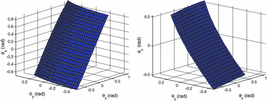
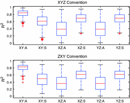
Fig. 7.4

The relationships between the X and Y components of the XYZ Euler angles and the ankle and subtalar joint displacements when the axis tilt angles of the ankle kinematic model are identical to those presented in the literature

Fig. 7.5

Box plots for R ² values found by fitting a linear model through the Euler angle–joint displacement relationships over 500 randomly generated model parameters. The top plot shows the R ² values for relationships obtained using various pairwise combinations of the XYZ Euler angles, while the bottom plot shows the same obtained using different pairwise combinations of the ZXY Euler angles. Note that the notation of P:Q is used to identify results relating to the angle pairing P and displacement output Q, with A and S denoting the ankle and subtalar joint displacements, respectively

Only gold members can continue reading. Log In or Register to continue