Functional Biomechanics of Healthy, Anterior Cruciate Ligament-Deficient and -Reconstructed Knees

Kevin B. Shelburne

Marcus G. Pandy

Michael R. Torry

Prelude

Musculoskeletal biomechanics has the potential to make significant contributions to medicine, ergonomics, and sports performance. The study of human motion (kinesiology) is especially relevant, as it is segment motions and the interaction of the muscles and external forces that can cause the acute and/or chronic breakdown of physiologic tissue. Moreover, it is the extraordinary adaptability of the body that allows for continued activity, even in the presence of an injury or pathology. In the anterior cruciate ligament (ACL)-deficient knee, for instance, many individuals suffer through instability and episodes of giving way in an effort to remain physically active, only to be faced later on with meniscal damage and the development and progression of osteoarthritis. Equally, some individuals appear to compensate very well with an ACL deficient knee, as they appear to effectively utilize muscular strategies to stabilize the knee during activities.

This chapter focuses on the understanding of normal knee function and the biomechanics of the ACL-deficient and ACL-reconstructed knee during activities of daily living. Basic experiments concerning the performance adaptations
in the ACL-deficient and ACL-reconstructed knee will be reviewed, and the biomechanics of the normal, ACL-deficient, and ACL-reconstructed knee under more strenuous activities, such as landing from a jump, will also be provided. By combining information obtained from two distinct but related scientific disciplines (in vivo experimentation and computer modeling), much of our work in recent years has focused on describing and explaining the intra-articular loads that occur at the knee.

Background: Computer Simulation and In Vivo Measurement of Human Motion

The lower extremity musculoskeletal system is composed of a series of jointed links (segments) that can be approximated as rigid bodies. Six independent parameters (the degrees of freedom) are required to describe the location and orientation of each of the lower extremity body segments in three-dimensional (3D) space. In vivo measurements quantitatively describe the spatial motion of these segments and the movements of the joints connecting these segments over time and during dynamic motions. Historically, in vivo measurements of lower extremity mechanics for dynamic activities have been acquired with optical capture, accelerometer, or goniometric methods. The most common of these are the optical systems that employ high-speed cameras to capture the 3D motion of reflective markers that are placed on the limb segments and pertinent bony landmarks of the subjects. These systems produce 3D trajectories of the markers, which are used to estimate the position, velocity, and acceleration of the body segments during the activity. These kinematic parameters are then combined (in a process termed the inverse dynamic solution) with a subject’s anthropometric measurements and external forces (commonly measured with a force-plate mounted in floor) to yield external reaction forces and net moments at the joints. The internal muscle contraction, passive soft tissues, and joint-reaction forces must generate equal and opposite forces to the externally measured moments and forces. These methods have been applied to a myriad of sporting motions and pathologic diseases. Yet, despite their widespread use in orthopaedic research, this technology cannot determine muscle forces and/or forces borne by the individual ligaments and other tissues. Without this information, specific conclusions regarding tissue loads are not possible.

To remove this limitation, scientists have developed sophisticated computer simulation techniques that estimate loads in the muscles and on specific tissues and intra-articular structures. Quite simply, computer simulation allows for the estimation of forces in specific tissues that cannot otherwise be measured in vivo. A computer simulation is based on a mathematical model of a biological system that represents the geometry, anthropometry, and mechanical material properties of the tissues. Put simply, a musculoskeletal model of the body represents the bones, joints, muscles, and ligaments of the body. With today’s computing technology, these models can often be visualized in 3D with moderately powered computer workstations. Because all models are simplifications of reality, there is always a trade-off between level of detail and computational complexity. Although models represent the physical properties of a system, a simulation applies conditions (such as the joint motion and external loads from walking) to the model and calculates the resultant motion and loads. Thus, a simulation generally refers to a computerized version of the model, which is used to study the muscle, ligament, and joint loads of a defined motion.

In vivo measurements and computer simulations form a continuous cycle of investigation (Fig. 17.1). Most often, investigation of a particular activity, condition, or pathology begins with laboratory measurements. In application to the knee and its function during activities of daily living and sporting motions, this means measurement of body segment kinematics, joint moments, external forces, and appropriate muscle electromyography (EMG) activations in subjects. Then, in order to understand the loads inside the body, the experimental data are used to develop a computer simulation. The outputs of the simulation are often the muscle forces, joint loads, and ligament loads during the measured activity. In many cases, the computer simulation yields results that lead to additional focused laboratory experiments. This process continues with refinement of the experimental and simulation methods until an adequate level of understanding is developed. In this way, experiments and simulation coexist as disciplines for developing a level of understanding of the interaction of all the individual parts of a system, and of the system as a whole.

In the following review of knee function, much of the scientific detail regarding the in vivo experimental methodology as well as the construction and performance of the computer simulations are omitted but are adequately referenced so that the reader may refer to the peer-reviewed articles for a detailed description of the specific methods.

Knee Function and Loads During Activities of Daily Living

Quantifying ligament loads at the knee during activity is motivated by the high incidence of knee ligament injuries, the frequency of their surgical treatment, and the subsequent rehabilitation protocols. In addition, onset and progression of knee osteoarthritis is often attributed to an injury or pathology that alters the way the knee carries force. Little is known about the way muscles, ligaments, and external forces contribute to loading of the knee joint during activities of daily living. Forces in the ligaments and between the bones are determined mainly by the forces in the muscles and the external loads on the
lower limb that accompany activity. Because these loads are large and specific to each activity, in vitro simulation of knee loading with cadaveric limbs is often insufficient to represent the in vivo loading environment of the knee. The following sections describe knee mechanics for a variety of activities of daily living and sport. Each activity is treated separately because the forces borne by the knee cannot be generalized from one activity to another.

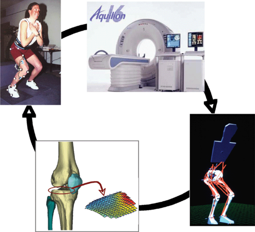Figure 17.1 In vivo experiments conducted in the laboratory can provide a wealth of information on how a person performs a motion, but these methods cannot provide information about intra-articular loads. Computer modeling can predict these loads. These two disciplines work in continuity as computer models require in vivo data such as kinematics, ground-reaction force, and kinetics for comparison and model validity. This is illustrated above in which experimental data (upper left figure) is collected, then subject specific joint geometry is collected (upper right picture) using MRI and/or CT. These techniques provide modelers with the basic data to create realistic models and foward dynamic simulations (bottom right picture) by which intra-articular loads can be estimated (bottom left picture). Together, these techniques provide a very powerful tool in the understanding of human function and its consequences on tissue structure. (All photos contained in this figure are courtesy of Marcus G. Pandy, University of Melbourne, Melbourne, Australia; and Michael R. Torry and Kevin B. Shelburne, Steadman Hawkins Research Foundation, Vail, CO).

Knee Flexion and Extension

Much attention has been given to understanding ligament function during flexion/extension of the knee. The reasons for this are that these can be well-controlled experiments and often form part of the rehabilitation protocol following knee injury. Knee flexion/extension with and without resistance forms part of many rehabilitation protocols following ligament injury or repair, and although conceptually simple, understanding the behavior of the knee during knee flexion and extension can enlighten the function of the knee ligaments during more demanding activities of daily living and sport. Shelburne and Pandy¹ used a computer simulation of knee flexion/extension to study ligament forces induced by isolated contractions of the extensor and flexor muscles with the specific goals of predicting the forces induced in the ACL and posterior cruciate ligament (PCL) and to explain how these forces were influenced by knee angle and the geometry of the knee tissues.

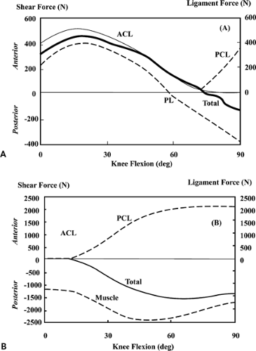Figure 17.2 A: Anterior-posterior shear forces applied to the tibia (thick line) and resultant cruciate ligament forces (thin line) for a maximum isometric knee extension. Total shear force (thick solid line) represents the resultant shear force applied to the tibia and is equal and opposite to the net shear force supplied by all ligaments and capsular structures. B: Anterior-posterior shear forces applied to the tibia (thick line) and the resultant cruciate ligament forces (thin line) for maximum isometric knee extension. Muscle (thick line) represents the total shear supplied by the hamstrings and gastrocnemius. Hamstrings dominate the curve, with gastrocnemius only contributing less then 10% at all angles of knee flexion. ACL, anterior cruciate ligament; PCL, posterior cruciate ligament; PL, patellar ligament/tendon. (Reproduced with permission from

Shelburne KB, Pandy MG. A musculoskeletal model of the knee for evaluating ligament forces during isometric contractions. J Biomech 1997;30:163–176.

)

Results indicated that the ACL is loaded from full extension to approximately 80 degrees of flexion during maximum, isolated contractions of the quadriceps (Fig. 17.2A,B). This suggests that quadriceps exercises should be limited in this region if the ACL is to be protected from load. In contrast, isolated hamstring and gastrocnemius muscle contractions will protect the healing ACL graft throughout the entire range of knee flexion. The study also showed that the ACL cannot be protected from all load in the 0- to 10-degree range irrespective of any combination of hamstring, gastrocnemius, and quadriceps muscle activations as the ACL load in this range is determined mainly by the line of action of the ACL in relation to the shapes of the articulating surfaces of the medial and lateral compartments. As the knee flexes beyond 10 degrees, ACL load can be lowered by decreasing quadriceps activation or by increasing hamstrings activation. This is because the pattern of ACL loading in this range is governed by the geometry of the patellofemoral joint and the mechanical properties of the hamstrings. As the knee flexes, the angle between the patellar tendon and the long axis of the tibia also decreases. As this angle decreases, so does the shear force supplied by the patellar tendon. ACL force decreases in proportion to the decrease in patellar tendon shear force because the ACL is the primary restraint to this force. In addition, the angle between the hamstrings and the tibia increases. Thus, the amount of shear force provided by the hamstrings increases because of geometry alone. In short, for a constant quadriceps and hamstrings force contraction, ACL force decreases monotonically as the knee flexes.

Rehabilitation following ACL injury or repair is often associated with knee extension exercises that also employ external loads (isometric, isokinetic, and isotonic knee extensions). Pandy and Shelburne² evaluated the influence of muscle activity in conjunction with an external restraining force (i.e., a tibial push pad as used in Cybex [Cybex, Inc, Ronkonkoma, NY] testing) on the forces induced in the knee ligaments during isometric knee extension exercises. Moving the tibial restraint closer to the flexion axis decreases the ACL load because it increases the amount of posterior shear force applied to the tibia by the pad. The study found that the ACL force is practically independent of the orientation of the restraining force. This means, at all angles of isometric loading, that decreasing the angle
between the line of action of the restraining force and the long axis of the tibia has only a small effect on ACL loading.

Several studies have documented an increase in anterior tibial translation in the ACL-deficient knee during knee extensions. However, the numerous in vitro studies conducted in this area may be limited as ligament function in cadavers may be different compared with that of in vivo ligaments and because the muscle loads applied to cadavers are often much less than the muscle loads used during ordinary activities. Pandy and Shelburne² showed that anterior laxity in the intact knee is greatest between 20 and 30 degrees and the primary restraint to anterior tibial translation is the ACL, which provides 85% to 95% of the total restraining force. Anterior laxity increases when the ACL is removed. The greatest increase occurs between 15 and 30 degrees relative to the intact condition. The deep fibers of the MCL become more loaded during an anterior drawer providing up to 80% resistance to anterior tibial translation and this remains consistent throughout all flexion angles.

Even though anterior tibial translation increases in ACL-deficient knee extension, the extensor torque remains more or less the same relative to the intact knee. This is because the patellar tendon force and the moment arm of the patellar tendon do not change when the ACL is torn. In general, this analysis suggests that the knee extensor mechanism does not change much in the absence of the ACL as the force transmitted to the patellar tendon, the location of the flexion axis, the moment arm of the extensor mechanism, and the torque developed by the quadriceps are all nearly the same as compared to the intact knee. This is because the change in line-of-action of the patellar tendon relative to the rotational center of the knee changes little with increased anterior tibial translation. However, the decrease in patellar tendon angle relative to the long axis of the tibia reduces the anterior shear force applied to the shank. For this reason, although MCL force increases, MCL force in the ACL-deficient knee remains much lower than that found in the ACL in the intact knee under identical external and muscle loads. This is an important factor in the later description of ACL-deficient walking.³

Collectively, these data suggest that the performance differences often observed in ACL-deficient knees are a result of quadriceps strength deficits and not from an increase in anterior tibial translation. In addition, although function of the knee extensor mechanisms is not altered by loss of the ACL, the load sharing amongst the ligaments is substantially different; the deep fibers of the medial collateral ligament (MCL) bear nearly all the resistance to anterior tibial translation and the tibiofemoral joint load is carried farther posterior on the tibial plateau. These findings support the clinical observations of increased MCL and medial meniscal injuries in the ACL-deficient knee.

Knee Bends and Squatting

The previous discussion has focused on nonweightbearing knee extension exercises. However, weightbearing exercises such as squatting or “knee dips” are most often prescribed for post-ACL repairs. As with the knee extension exercise, very little experimental data are available because it is difficult to measure ACL loads in vivo; although these loads have been estimated using cadaveric specimens and are thought to be low, the muscles forces that are used in those studies are much lower (five to eight times lower) than what are actually occurring during the exercise.

In 2002, Shelburne and Pandy⁴ investigated the squatting motion using a forward dynamic model based on optimization theory. In this simulation, the ACL was loaded from 15 to 40 degrees of knee flexion but the peak force in the ACL only reached a maximum of 20 N. The PCL was loaded at flexion angles greater than 30 degrees and reached a maximum value of 66 N at 81 degrees. Peak MCL force reached 40 N, which is roughly the same loads as reported during passive knee extension movements. The quadriceps developed nearly 3,000 N of force as the knee approached 80 degrees; compared to the maximum hamstring forces, which reached 500 N. The pattern of muscles forces created a similar pattern of tibiofemoral and patellofemoral loading and is representative of the acceleration of the body up from its squat position. The tibiofemoral and patellofemoral loads during squatting are much less than those occurring at the knee during active knee extension exercises. For comparison, during isometric, maximal contractions, tibiofemoral and patellofemoral loads are estimated at 6,000 and 10,000 N, and for the sit-to-stand motion these were estimated at 2,800 and 3,200 N, respectively. The results of Shelburne and Pandy⁴ generally support the view that weightbearing, squatting exercises can be a relatively safe exercise following ACL repair.

Walking

Ligament Loads During Walking

Walking is one of the most common and basic of human movements. Although we usually take this motion for granted, it is one of the most complex and integrated motions all able-bodied persons do on a daily basis. It has been well described and scientifically analyzed in hundreds of laboratories throughout the world. This is important because a large body of data now exists by which standards and norms can be compared with pathologic conditions with ease. This allows for even the smallest deviations from normal gait patterns to be informative to the knowledgeable and discerning clinician.

A number of studies have inferred ACL loading from in vivo measurements of bony motion at the knee,⁵^,⁶^,⁷ but very few studies have calculated knee-ligament forces in gait. Of those that have, there appears to be some disparity in the results. Morrison⁸ used an inverse dynamics approach to estimate muscle, ligament, and joint contact forces at the knee during normal, level walking. His calculations showed that the ACL was loaded throughout the stance phase of walking, and that peak ACL force was 156 N
(approximately one-fourth body weight [BW]). Using a similar approach, Harrington⁹ also found that the ACL was loaded throughout stance, but the peak force transmitted to the ligament was estimated to be much higher (approximately one-half BW).

In 2004, Shelburne et al.³ using a 3D model of the lower limb (Fig. 17.3) and knee, described cruciate ligament forces during walking in terms of the shear force applied to the knee. The ACL was loaded throughout the stance phase of gait (Fig. 17.4). Peak ACL force occurred at contralateral toe-off and was estimated to be 303 N, which is about 13% of the reported failure strength of the ligament¹⁰ and is similar to the levels of ACL loading predicted for isokinetic knee-extension exercise at fast speeds.¹¹^,¹² The force induced in the ACL was explained by the balance of muscle forces, joint contact forces, and the ground-reaction force
applied to the leg; each of these forces contributed to the resultant shear force acting at the knee. The patellar tendon, gastrocnemius muscle, and tibiofemoral contact force all applied anterior shear forces to the leg, while hamstrings and the resultant ground-reaction force applied posterior shear forces (Fig. 17.5).

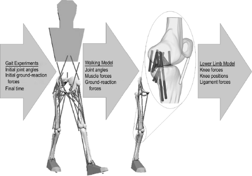Figure 17.3 Schematic of the forward dynamic walking model used to determine individual muscles forces during the gait cycle. Muscle forces, ground-reaction forces, and lower limb motions obtained from the walking simulation matched experimental measures in the laboratory. These parameters were then input into a lower limb model. Ligament forces and joint contacts loads were then estimated using the three-dimensional model of the knee joint. (Reproduced with permission from

Shelburne KB, Torry, MR, Pandy MG. Muscle, ligament, and joint-contact forces at the knee during walking. Med Sci Sports Exerc 2005;37:1948–1956.

)

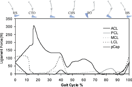Figure 17.4 Forces in the cruciate ligaments (ACL, anterior cruciate ligament; PCL, posterior cruciate ligament), collateral ligaments (MCL, medial collateral ligament; LCL, lateral collateral ligament), and the posterior capsule (pCap) of the knee during one complete gait cycle. HS, heel strike; CTO, contralateral toe-off; CHS, contralateral heel strike; TO, toe-off. Peak force in the ACL coincided with peak knee extensor torque and quadriceps muscle forces. (Reproduced with permission from

Shelburne KB, Pandy MG, Anderson FC, et al. Pattern of anterior cruciate ligament force in normal walking. J Biomech 2004;37:797–805.

)

In early stance, the shear force from the patellar tendon dominated the resultant shear force applied to the leg, and so maximum force was transmitted to the ACL at this time (Fig. 17.5). Patellar tendon shear force was large in early stance because quadriceps force was large and also because the line of action of the patellar tendon was inclined anteriorly relative to the long axis of the tibia.¹^,¹¹ ACL force was relatively small in late stance because the posterior component of the ground-reaction force was nearly equal to the sum of the anterior shear forces supplied by the patellar tendon, gastrocnemius muscle, and the tibiofemoral contact force at that time (Fig. 17.5). Gastrocnemius applied an anterior shear force to the shank because the knee was nearly fully extended just before contralateral heel strike, and at small flexion angles the gastrocnemius wraps around the back of the tibia.¹^,¹¹^,¹²^,¹³ Tibiofemoral contact force applied an anterior shear force to the leg because of the posterior slope of the tibial plateau.²^,¹¹^,¹⁴ The ground-reaction force applied a posterior shear force to the leg because the line of action of the resultant ground force passed behind the knee. The posterior shear force caused by the ground reaction increased prior to contralateral heel strike because the angle between the shank and the ground increased at this time.

The model PCL was unloaded during stance because the resultant shear force at the knee pointed anteriorly at this time (Fig. 17.5, shaded region). This result of the model correlates with the clinical observation that the knee often responds adequately to conservative treatment after isolated rupture of the PCL, without the need for reconstruction.¹⁵^,¹⁶

Peak force borne by the MCL was less than 20 N during stance (Fig. 17.4). The model MCL was not loaded much for two reasons: first, the ACL provided the primary restraint to anterior tibial translation in the intact knee; and second, the ground-reaction force applied an adductor moment to the leg, which could only be resisted by the structures on the lateral side of the knee. The study by Shelburne et al.³ showed that the muscles that applied the largest forces at the knee during walking were the vasti and gastrocnemius. Peak force in vasti was 1,188 N, which occurred at contralateral toe-off. Peak force in gastrocnemius was lower at 849 N, and it occurred at contralateral heel strike. The hamstrings developed much lower forces during stance; peak force predicted for hamstrings was 495 N, which occurred at heel strike.

The model calculations showed a bimodal pattern for patellofemoral and tibiofemoral contact force (Fig. 17.6A,B), with the first and second peaks of tibiofemoral load aligning with peak forces developed by the quadriceps and gastrocnemius muscles. The calculations also showed that the center of pressure at the knee was concentrated on the medial side. Compressive force acting between the femur and tibia was much greater in the medial compartment than in the lateral compartment throughout the stance phase of gait. The compressive force was much greater on the medial side because the resultant ground-reaction force passed medial to the knee at all times during
stance. The medially directed ground-reaction force created an external moment that acted to adduct the knee in the frontal plane.¹⁷^,¹⁸

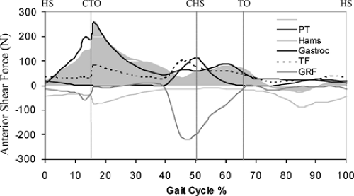Figure 17.5 Shear forces acting on the leg (shank + foot) during the simulated gait cycle. The shaded region shows the total shear force borne by the knee ligaments in the model. Total shear force is the shear force due to the muscle forces, ground-reaction forces, and joint contact forces. Anterior shear forces (+ values) tended to translate the leg anteriorly; posterior shear forces (− values) tended to translate the leg posteriorly. Hamstrings always applied a posterior shear force. The ground-reaction force applied a posterior shear force to the leg because the line of action of the resultant ground force passed behind the knee. HS, heel strike; CTO, contralateral toe-off; CHS, contralateral heel strike; TO, toe-off; PT, patellar tendon; Hams, hamstrings; Gastroc, gastrocnemius muscle; TF, tibiofemoral contact force; GRF, ground-reaction force.). (Reproduced with permission from

Shelburne KB, Pandy MG, Anderson FC, et al. Pattern of anterior cruciate ligament force in normal walking. J Biomech 2004;37:797–805.

)

The adduction moment is considered a key determinant of the distribution of tibiofemoral load between the medial and lateral sides of the knee (Fig. 17.7A). The external knee adductor moment was resisted by a combination of muscle and ligament forces.¹⁹ The quadriceps provided most of the resistance in the first half of stance, while the gastrocnemius contributed most of the resisting muscular moment thereafter (Fig. 17.7B).¹⁹

Ligaments provided significant resistance to the external knee adductor moment immediately after heel strike and during midstance (Fig. 17.7C). Schipplein and Andriacchi¹⁸ found that the adductor moment was resisted by the passive lateral supporting structures of the knee for nearly 60% of the stance phase of gait. The contribution of ligament to resist adduction moment during walking was highest when muscle force (and muscular flexion-extension moment) was lowest.

The posterior lateral capsule (PLC), which was represented by the lateral collateral ligament and the popliteofibular ligament, provided the primary passive restraint to lateral joint opening in the model (Fig. 17.7C).¹⁹ Peak forces borne by the lateral collateral ligament and popliteofibular ligament were 167 and 15 N, respectively. Although the peak force borne by the ACL in the model was much higher than that calculated for the PLC, the ability of the ACL to resist the external adductor moment at the knee was much less.¹⁹

The pattern of force calculated for the PLC was similar to that obtained for the external adductor moment at the knee. PLC force was highest at times when the external adductor moment was high and the resistance provided by the muscles was low. This is consistent with results obtained from cadaveric experiments, which show that the PLC plays an important role in resisting adductor moments applied at the knee.¹⁹

Only gold members can continue reading. Log In or Register to continue