Parameters that are commonly extracted from studies
Characteristics of the manuscript
Author
Publication year
Study duration
Study design
Factors related to risk of bias
Participant characteristics
Number
Age
Sex
Diagnosis/criteria used for diagnosis
Ethnicity
Disease duration
Predisposing factors to the condition that is being assessed
Characteristics of the intervention and comparator
Dose
Frequency
Mode
Duration
Timing
Characteristics of the outcomes
How the outcome is defined
The unit of measurement
Upper and lower limits of normal for laboratory parameters
Time from baseline that the outcome is evaluated
Others
How the missing data is handled
Outcomes of specific subgroups
The data extraction should also ideally be performed by two independent observers. Just like the clinical report forms (CRF) that one would use in clinical trials, it is important to have standard forms for data extraction in order to make the process homogenous and keep track of missing data.
Summarizing the Data and (if Possible) Pooling (Meta-analysis)
It is not uncommon for a systematic review to yield articles which show substantial heterogeneity in methodology and results which make it impossible to pool the data and perform a meta-analysis. If this is the case, usually results of the individual trials are summarized with emphasis on their characteristics and potential biases.
If it is reasonable to pool and combine the data from individual studies statistically, then meta-analysis can be performed. The type of data, in terms of being continuous or dichotomous, and its heterogeneity are factors that need to be considered when deciding which statistical methods will be used for the meta-analysis. These will be further discussed in the following sections.
Reporting the Results
The PRISMA statement provides a guideline for reporting systematic reviews and meta-analyses to achieve a standard in manuscripts [19]. It is very important to report the number of studies which are identified by the literature search in each of the databases or other sources, number of articles that had been screened and excluded after reading the title and the abstract as well as the articles that are excluded after reading the full text and the reasons for excluding them.
The possible factors that may affect the outcome of the studies, assessed by quality or risk of bias assessment and results of the sensitivity analysis, should also be reported.
The reliability of the result of the meta-analysis is evaluated by the GRADE approach in Cochrane reviews. Here the reliability of the results is graded in four levels from very low to high, depending on whether the evidence is coming from studies with the preferred study design, the presence of factors decreasing the quality of evidence such as limitations in the design of included studies, inconsistency of results, indirectness of evidence, imprecision and publication bias and the presence of factors which increase the quality of evidence, such as large magnitude of effect or dose–response gradient, which are mainly used for evaluating observational studies. It is important to provide some form of evaluation of the reliability of the results to help the readers to be able to interpret the results correctly.
Choice of the Effect Parameter
Once the article data are extracted, the first step in the meta-analysis is the choice of the effect parameter. There are several possibilities. If the outcome variable is continuous, for instance the decrease in a depression score during treatment, then a straightforward choice would be the difference between the mean decrease in the experimental treatment group and that in the control group. When the absolute difference between the means is difficult to compare between the studies, for instance if depression is rated by different instruments across studies, usually the standardised difference is chosen, which is the difference between the group means divided by (mostly) the pooled standard deviation at baseline. This means that the difference between the groups is expressed in the number of standard deviations. When the standard deviation or standard error with the sample size is known for each treatment group, the 95 % confidence intervals (CI) can be calculated. It is customary to present the 95 % CIs of all studies in a figure called the forest plot. This plot provides a first impression of the evidence in favour of an effect of the experimental treatment relative to the control treatment.
In case of a dichotomous outcome variable, like for instance, the patient does or does not respond to a treatment, the data for each study can be represented in a 2 × 2 table. Then the treatment effect can be characterised by either the odds ratio (OR), the risk ratio (RR, also called the relative risk) or the risk difference (RD). As an example, we take a meta-analysis reported by Gârces et al. [20]. They investigated the effect of antidrug antibodies (ADA) on drug response (positive or negative) to antitumour necrosis factor (aTNF) biological therapies. In Table 2, the extracted data are given. There are 13 studies, and for each of them, the number of responding patients and the total number of patients are given for the ADA-positive and ADA-negative group separately.
Table 2
Extracted data
Patients with aTNF response/total no. of patients | ||
|---|---|---|
Study | ADA positive | ADA negative |
1 | 0/10 | 24/24 |
2 | 1/5 | 22/25 |
3 | 9/21 | 76/100 |
4 | 4/13 | 2/2 |
5 | 3/13 | 13/16 |
6 | 4/18 | 17/17 |
7 | 1/11 | 20/27 |
8 | 8/22 | 20/29 |
9 | 3/23 | 56/62 |
10 | 0/7 | 10/13 |
11 | 4/7 | 23/24 |
12 | 1/10 | 37/41 |
13 | 2/6 | 20/23 |
Given the choice of the effect measure (RD, OR or RR), a 95 % CI is calculated with the usual formulas, and these are presented in the forest plot. In practice, one of the three possible effect measures is taken, but here we show for illustration all three forest plots (Fig. 1). The confidence intervals are made in the usual way, taking estimate ±1.96 × standard error.
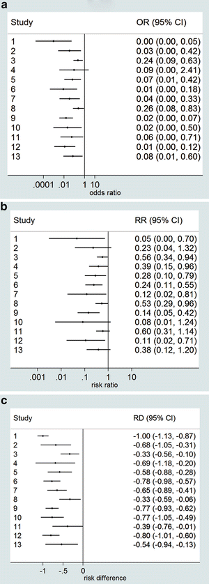

Fig. 1
These figures have been made with the meta-analysis package of Stata [21]. The program employs the usual approximate formulas for the confidence intervals, which can be somewhat inaccurate if the number of responding or non-responding patients is small. This is the case here for some of the studies, and the confidence intervals of these studies are therefore rather inaccurate, as is illustrated by some studies having a confidence interval for the RD that exceeds the value −1, which is impossible since a difference between two proportions cannot exceed 1 in absolute value. Some programs are able to calculate better confidence intervals in the case of small numbers.
Notice that the ratio measures are represented on a logarithmic scale, which is customarily done for ratio measures. The advantage of the logarithmic scale is that the CIs are symmetric and that the figure does not essentially change visually if the numerator and denominator are interchanged. As an illustration in Fig. 2, we have given the forest plots for the RR on the non-logarithmic scale. Figure 2a gives the RR of the ADA-positive group relative to the ADA-negative group, while Fig. 2b shows the RR of the ADA-negative relative to the ADA-positive group.
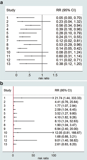

Fig. 2
(a, b) Forest plots for the RRs of the meta-analysis data of Table 2. (a) RR of response in ADA-positive versus ADA-negative group and (b) RR of response in ADA-negative versus ADA-positive group
Notice that the confidence intervals are very asymmetric and the figures look much less attractive than Fig. 1b. Some of the confidence intervals in Fig. 2b do not even fit within the figure. Furthermore, Fig. 2a, b look very different, while essentially they are the same since it is arbitrary what to take as the numerator or denominator of the risk ratio.
In the rest of this chapter, we take the RR as the effect measure. All methods discussed are equally applicable to other choices for the effect measure.
Meta-analysis
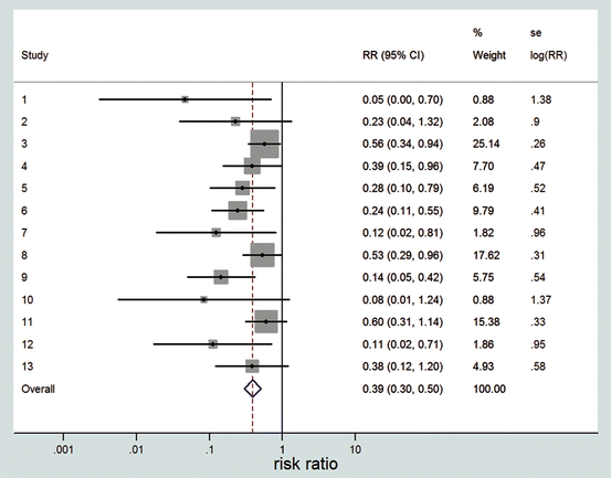
The forest plot in Fig. 1b is very nice in the sense that it gives a complete description of all the available data. In this case, the overall conclusion, at least qualitatively, is clear. On the average, there is definitely an effect of ADA positivity on the response to anti-TNF treatment. However, the conclusion is not always this clear in meta-analyses. In addition, we would like to answer more specific questions such as: What is the overall (average) effect across studies? What is the corresponding confidence interval? Is the overall effect statistically significant? Is there variability in the effects across studies, and if so, how large is it? The meta-analysis answers these types of questions as well. Sometimes the meta-analysis is also called “pooling the data”, but this does not mean that all data are simply thrown together, in one 2 × 2 table. To carry out a meta-analysis, all that is needed is the estimated effect and its standard error per study. The method of analysis is independent of the specific choice of the effect measure.
Fixed-Effect Meta-analysis
The starting point is the availability of the effect estimate and its standard error for each study. It is important to realise that the observed effect in a study is not the true value of the effect in that study, but only its estimate. The true effect of a study would only be known if the study had an infinitely large sample size. Due to sampling variability, the observed effect deviates from the true effect. The studies are called homogeneous if it is reasonable to assume that all true effects are equal across studies. In that case, since there is one common effect to all the studies, the meta-analysis is called a fixed-effect analysis. The first question is how to make an estimate of the value of the common treatment effect? It is tempting to just take the simple mean of all observed effects. However, larger studies are more informative than smaller studies, as is reflected in smaller standard errors. Thus, we should better calculate a weighted mean instead of a simple mean, such that the larger studies have a larger weight. Statistical theory says that the optimal weights are equal to the inverse squared standard errors. So, if a study has a two times smaller standard error than another study, then the first study should count four times as heavy as the second. Weighting by the inverse squared standard errors is often very similar to weighting by the total sample sizes. For ratio measures, the calculations are done on the logarithmic scale and translated to the original scale afterwards. In Fig. 3, the resulting overall estimate of the RR in our example is given as 0.39. It means that the probability to respond for ADA-positive patients is 0.39 times the probability to respond for ADA-negative patients, or, in other words, the probability to respond is reduced by 61 % in ADA-positive patients compared to ADA-negative patients.
