Olecranon apophysis morphology
Skeletal age (Y)
Girls
Boys
Two ossific centers
11
13
Half-moon image
11.5
13.5
Rectangular aspect
12
14
Beginning of fusion
12.5
14.5
Complete fusion
13
15
The main disadvantage of the Sauvegrain method is the limited use to the pubertal phase and the year preceding it (10–13 years and 11–14 years in girls and boys respectively). Prior to the pubertal phase, the elbow is largely cartilaginous and changes in the ossific centers cannot be clearly differentiated (Fig. 46.1).
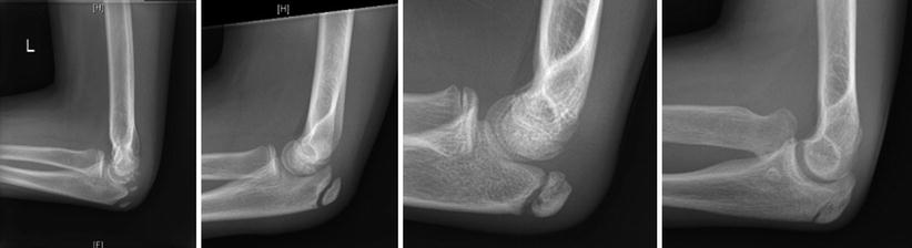
Fig. 46.1
Sauvegrain skeletal bone age
The shorthand bone age assessment method developed by Heyworth et al. [29] was to simplify the determination of skeletal age by using a single radiographic criterion from Greulich and Pyle atlas for males between the ages of 12.5 to 16 years and females from 10 to 16 years (Table 46.2). Good intraobserver and interobserver reliability was reported in assessing bone age of 140 males and 120 females. There was substantial agreement and strong correlation when compared with Greulich and Pyle assessments (Level III evidence).
Table 46.2
The shorthand bone age assessment method
Radiographic criteria | Skeletal age (Y) | |
|---|---|---|
Girls | Boys | |
Appearance of hook of hamate ossific nucleus | 10 | 12.5 |
Appearance of thumb sesamoid ossific nucleus | 11 | 13 |
Width of proximal aspect of distal radius epiphysis equals width of distal aspect of distal radius metaphysis, but has not yet begun to cap | – | 13.5 |
Capping of distal radius epiphysis | 12 | 14 |
Closure of thumb distal phalanx physis | 13 | 15 |
Closure index finger distal phalanx physis | 13.5 | 15.5 |
Closure of index finger proximal phalanx physis | 14 | 16 |
Closure of index finger distal metacarpal physis | 15 | – |
Closure of distal ulna physis | 16 | – |
Closure of distal radius physis | 17 | – |
Growth Tables and Charts and the Determination of Growth Percentiles
The first step in the prediction of the future growth remaining in a limb or a limb segment is to determine the growth percentile or the relative size for age (chronologic or skeletal age) within which this limb or limb segment would lie relative to the standard growth records. This is very important because an individual growth tends to be within the same growth percentile throughout different growth phases [23] and in turn would allow us to track and predict the future growth remaining along the records of his peers within the same percentile till skeletal maturity. The growth percentile can be assessed by using different available age and gender specific growth tables and charts which document the average values and percentiles [22, 23, 36, 37].
The most complete set of longitudinal records of height and lower extremity growth in children and the most commonly used growth database in clinical practice is that published by Green and Anderson [22, 23]. Green, Anderson and Messner published two landmark studies. In the first one [23], they used longitudinal data for femoral and tibial lengths of healthy children, recorded by annual lower extremity radiographs from 1 to 18 years of age (67 boys and 67 girls). Those growth data were for North American white males and females of predominately Irish origin and were collected as a part of a longitudinal series of child health and development studies conducted at Harvard School of Public Health, Boston from 1930 to 1956 [38]. They were able to construct gender specific growth tables and charts based on chronologic age from 1 to 18 years defining annual average growth values and standard deviations or growth percentiles (mean ± 1 and 2 SD). In a separate work [22], they published growth remaining charts and tables for the normal femur and tibia relative to chronologic and skeletal age of 50 boys and 50 girls between the age of 8 and 18 years. Forty-nine children (25 girls and 24 boys) had unilateral paralytic poliomyelitis which affected only one lower extremity and therefore data of the healthy side were used. All children had annual orthoroentgenograms for the recording of femoral and tibial lengths as well as hand and wrist radiographic assessment of the skeletal age according to Greulich-Pyle Atlas [22, 26]. They further calculated the annual growth contribution and the growth remaining in the distal femur and proximal tibia (71 % of the total femoral growth and 57 % of the total tibial growth respectively) according to the skeletal age. Growth remaining tables and charts for the normal distal femur and proximal tibia were derived based on the skeletal age between 8 and 17 years with annual average values and four percentile levels (90th, 75th, 25th and 10th) and those tables and charts were the bases of Green and Anderson growth remaining method in predicting the optimal timing of epiphysiodesis. Green and Anderson work became the bases of Moseley straight line graph [39] and Paley’s multiplier method [24].
Other racial specific growth charts and curves were developed by Pritchett and Bortel [37] for Scandinavian American children in Denver, Colorado, by Beumer et al. [36] for Dutch children in Rotterdam, Netherlands and by Ha et al. [40] for Korean children. Beumer et al. [36] studied the femoral and tibial growth data in 182 Dutch children by serial orthoroentgenograms from 1979 to 1994. They found significant differences in the length of the femur in girls aged 8–9 years and boys 10–15 years and in the length of the tibia in boys and girls between the ages of 6–16 years. The Dutch children tend to be taller compared to the data of Anderson et al. [23]. They developed the Rotterdam straight line graph RSLG which is similar but not identical to Moseley straight line graph based on their own growth data.
Growth Inhibition Rate and Pattern of the Affected Extremity
Fredric Shapiro published an important article [34] in which he retrospectively reviewed longitudinal data of 803 children with LLD followed by the growth study unit at Boston Children’s Hospital over a 40-year period (1940–1980). All patients in this series were assessed at least annually (or more often semi-annually), for a minimum 5 years either to skeletal maturity or to the time of bony surgery. The disease entities which were included were: proximal focal femoral deficiency (PFFD), congenital coxa vara and congenitally short femur, Ollier’s disease, physeal destruction, poliomyelitis, septic arthritic of the hip, fractured femoral diaphysis, hemangioma, neurofibromatosis, hemiplegic cerebral palsy, hemiatrophy or hemihypertrophy, juvenile rheumatoid arthritis and Legg-Calvé-Perthe’s disease (LCPD). Shapiro was able to describe five main basic developmental patterns for progressive lower extremity length discrepancies (Table 46.3 and Fig. 46.2).
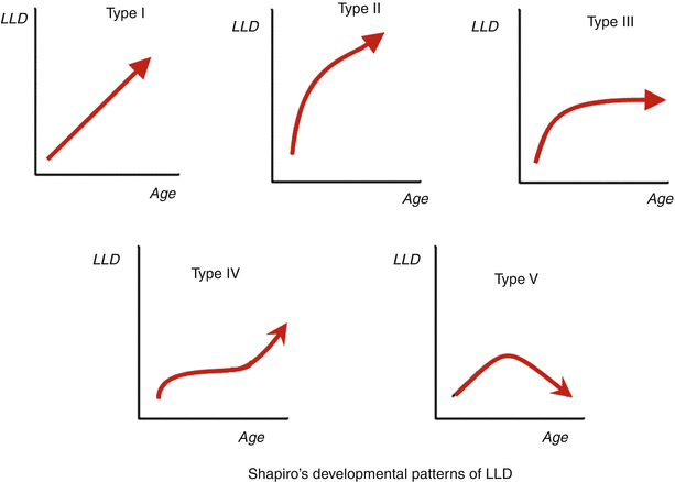
Table 46.3
Developmental patterns of lower extremity length discrepancies according to Shapiro
Type | Description | Common disease entities |
|---|---|---|
Type I – upward slope pattern | The discrepancy increases at a constant rate as the growth inhibition rate remains the same throughout growth | Congenital diseases like PFFD, physeal destruction |
Type II – upward slope-deceleration pattern | The discrepancy increases at a constant rate for a variable period of time and then shows decremental rate of increase which is variable from patient to patient and from condition to condition | Poliomyelitis, Juvenile rheumatoid arthritis |
Type III – upward slope-plateau pattern | The discrepancy increases with time and then a plateau is reached and it will not change throughout the remaining growth | Overgrowth following femoral fractures, Infections like diaphyseal osteomyelitis |
Type IV – upward slope-plateau-upward slope pattern | The discrepancy increases then stabilizes for a variable period of time and then increases again towards the end of growth | Hip disease (septic arthritis of the hip, LCPD, AVN with the treatment of DDH) |
Type V – upward slope-plateau-downward slope pattern | The discrepancy increases and then stabilizes and then decreases without surgery | Juvenile rheumatoid arthritis |
Fig. 46.2
Shapiro’s developmental patterns of LLD
The calculation of the predicted LLD is easiest with type I discrepancies which increase at a constant rate during the whole growth. In other words, the percentage of the length achieved by the short limb relative to the healthy side at any age would be the same during the remaining growth and therefore, the first step is to determine the length percentile of the normal bone or limb and calculate its final length at maturity for that percentile. The short limb length is then easily calculated as a percentage of the normal side maturity length. Type II is a difficult pattern to project as the information available from the period of constant increase before the deceleration phase has no predictive value. Multiple assessments for the growth inhibition rate are needed to allow for additional calculations. An example of type II discrepancies is poliomyelitis in which there is a tendency for the discrepancy to increase most rapidly in the first four or five years following infection then the rate of increased discrepancy diminishes gradually thereafter. In type III patterns, once a plateau has reached, the LLD will be the same throughout the remaining growth. The typical example for type III LLD is the overgrowth following femoral shaft fractures. Type IV discrepancies were found to be characteristic for hip diseases in childhood. Premature closure of the proximal capital femoral epiphysis is the cause for the late upward slope following a long time of plateau phase and once detected, it is easy to calculate the remaining growth of the entire femur and to add a 30 % from that value (the contribution of the proximal femoral physis the normal femoral growth) to pre-existing discrepancy to give the final LLD. In type V, the discrepancy starts to correct itself. It is commonly seen in chronic inflammatory diseases which stimulates growth under 10 years of age and then causes premature growth cessation towards the end of growth.
Calculating LLD at Skeletal Maturity and the Timing of Epiphysiodesis
To calculate the predicted LLD at skeletal maturity, one should firstly know the growth percentile of the long or healthy limb. With the help of the standard growth curves, the length of the long limb can then be projected to skeletal maturity to get its final length. When the growth inhibition rate and pattern of the short limb are taken in account, the final length of the affected limb at maturity and therefore the LLD at skeletal maturity can be calculated.
Menelaus Rule of Thumb
Menelaus rule of thumb was a simplified approach to project the limb length discrepancy at maturity based on chronological age rather than skeletal age and it didn’t take in account the growth percentile of the individual. It was based on the assumptions of White and Stubbins [42] that the lower femoral physis will grow by 3/8 inch/year while the upper tibial physis will grow by 1/4 inch/year. He assumed that growth would stop at the age of 16 years in boys and 14 years in girls [41]. He studied the results of 53 epiphysiodeses in 44 children who had the timing of surgery calculated based on this assumption. At maturity, 52 % of this group had a residual LLD of ¼ inch, 41 % within ¾ inch and 7 % more than ¾ of an inch (level IV evidence).
Green and Anderson Growth Remaining Method
To use Green and Anderson method, firstly the normal leg length (the femoral and tibial length) is compared to the data reported by Anderson et al. [23] for the current age and sex to determine the current growth percentile. The leg length is then projected to skeletal maturity for that percentile group to predict its final maturity length. The short leg length at maturity can be known after calculating the growth inhibition rate from previous assessments [(Growth of the long leg – Growth of the short leg)/growth of the long leg] and applying the same growth inhibition rate to the future growth of the long leg.
The next step is to use the growth remaining charts and tables to estimate the effect of physeal growth arrest procedures on the final length of the limb within the same growth percentile and hence the optimal timing of epiphysiodesis [22].
Moseley Straight Line Graph
Moseley converted Green and Anderson growth curve of the normal limb into a straight line of 45 ° slope by shifting the data points along the x axis and altering the distance between the age scale on the x axis by a comparable amount [39]. Another important concept for the straight line graph is the addition of a nomogram relating leg length to skeletal age for each gender which would provide a mechanism for taking the child’s growth percentile into account in predicting at what lengths the growth of the legs will stop. The main advantage of using Moseley straight line graphs is that it can demonstrate and take in account the rate of growth inhibition of the affected limb in predicting LLD and calculating timing of surgery. Furthermore, he added three reference lines which represent the amount of growth inhibition to be caused by epiphysiodesis of the proximal tibial and/or distal femoral growth plates (28 % and 37 % of the total growth of the leg respectively). Moseley compared retrospectively the use of straight line graph with Green and Anderson growth remaining method [22] to predict the final LLD at skeletal maturity in 30 patients (Level III evidence). In a group of 23 children who had been followed up for more than 1 year prior to surgery, the mean error in predicting final LLD was 0.6 cm for the straight line graph compared to 0.9 cm with the growth remaining method and the difference was statistically significant. The accuracy of the straight line graph was even more striking with a mean error of 0.6 cm compared to 1.2 cm with the growth remaining method when the growth inhibition rate of the affected side was taken in account.
Paley’s Lower Limb Multiplier
Paley and coworkers [24] used the growth data of Anderson et al. [23] and divided the femoral and tibial lengths at skeletal maturity by the femoral and tibial lengths at different ages during growth for each percentile group to get an age and gender specific multiplier (M = Lm/L, where M is the gender- and age-specific multiplier, Lm is the bone or limb length at maturity, and L is the age-specific bone or limb length). Maresh [43] reported growth data of 175 children using roentgenographic measurements of femoral and tibial lengths, ranging in age from birth to skeletal maturity. Those data were included as well to complete the period from birth to one year of age. They further used growth data from 18 additional growth databases, 9 based on radiographic or clinical length measurements and 9 based on anthropological measurements of femoral and tibial bones. The multiplier derived from all those database were similar. Therefore, the multiplier method should be independent of growth percentile, regional, racial, ethnic and generational differences in growth as it represents the percentage of growth remaining [44, 45]. Whatever the race or eventual limb length will be at maturity, 50 % of growth remains in the lower limb at 4 years of age. Other advantages for Paley’s method is that it is very useful in very young children and in cases with no available previous radiographs [46]. The main limitation is that it can be used only in patients with Shapiro type I progression pattern [34]. Paley et al. [24] compared the accuracy of their method to Moseley straight line graph in predicting the final actual LLD in two groups of patients, an epiphysiodesis group of 16 patients and a limb lengthening group of 14 patients. The correlation coefficients of comparing the Moseley predictions and the multiplier predictions were excellent >0.9 in both groups. If a threshold of acceptable accuracy was set to ±1.5 cm in the epiphysiodesis group, 5 out of 16 predictions by Moseley method and one multiplier prediction fell out of this threshold (Level III evidence).
Which Growth Prediction Methods Is the Most Accurate?
Evaluation of the accuracy of the different methods used to predict final LLD at skeletal maturity was studied extensively by several authors [44–49].
Related posts:
 Evidence-Based Treatment of Flexible Flat Foot in Children
Evidence-Based Treatment of Glenohumeral Dysplasia Caused by Obstetric Brachial Plexus Injuries
Evidence-Based Treatment of Flexible Flat Foot in Children
Evidence-Based Treatment of Glenohumeral Dysplasia Caused by Obstetric Brachial Plexus Injuries
 Evidence-Based Treatment of Deformity in Multiple Osteochondromatosis
 Evidence-Based Management of Ankle Fractures in Children
 Private: Physeal Injury, Epiphysiodesis and Guided Growth
 Femoro-Acetabular Impingement in Children
Stay updated, free articles. Join our Telegram channel

Full access? Get Clinical Tree


