Peloton Dynamics in Competitive Cycling: A Quantitative Approach

Fig. 1.

Sayama’s algorithm for cohesive and separating forces.

We take the way of calculating separating and cohesive forces, with minor adjustments, from this model. We calculate an acceleration for each agent, based on its relative position to the others. However, this code calculates it taking into account any other agent inside $R_{i}$ , a vision radius. This way, vision is isotropic. As we are trying to model human behaviour, it is useful to tweak this so that we only take into account agents that could possibly be seen by a human, that is, contained inside a visual cone. We also want to take different scales of distance when calculating cohesive and separating forces. Cohesive force should be a long-range calculation, taking into account pretty much any other agent in the visual field, while separating forces should be more local, with only close agents being taken into account.

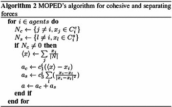
Based on these assumptions, we present the pseudo-code for these forces, defined here as Algorithm 2 (Fig. 2).

Fig. 2.

MOPEDs algorithm for cohesive and separating forces.

In Algorithm 2 (Fig. 2), $N_{c}$ and $N_{s}$ are, respectively, the neighbourhoods used for the calculation of cohesive and separating forces. These neighbourhoods are cones with an aperture angle of $140^{o}$ , defined to mimic a human visual cone, and different radii. The neighbourhood for cohesive force is being used with a radius of 20 m, and the separating one with a radius of 2 m, so that the rider only tries to avoid contact with other agents in the immediate neighbourhood.

A last point to be addressed in this section is some kind of bias to the center; real cyclists tend to be as close to the center of the road as possible in the case where no wind is blowing, so as to avoid danger on the fringes of the road. For that, a very small bias is put in place. Also, as in any flocking model, a small, random acceleration is put into place.

As a final addendum, we introduce the concept of active riders: a rider is considered active if he is willing to cooperate and be the frontrunner of the peloton, being out of drafting positions in order to protect the other cyclists. This is modelled by adding a small bias to the front for active cyclists, as far as they are not already the frontrunners.

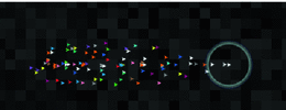
We observe that this algorithm, with the right set of parameters, yields a very life-like behaviour, with a narrow peloton front giving place to a wider formation behind, as it can be seen at Fig. 3.

Fig. 3.

View of a simulation of the peloton.

2.2 Energetic Parameters

We will now group together mechanical and physiological parameters, since both sets of parameters affect the energetic balance of the cyclist, making it easier to analyse them together.

Physiological data about cyclists is abundant; the literature on how the human body behaves under these circumstances is extensive and it is not our idea to redefine anything on this domain, but rather to use existing results and adjust our model to reflect them.

Many mathematical models for competitive cycling exist already. For this model, we will use elements from Olds [2], who has a validated, well-behaved set of equations for energy expenditures. We also use specific results from Hoenigman et al. [3], who extended Olds’ results and applied it on an agent-based model, and Martin et al. [8] for the potential-energy equation. By taking an agent-based approach and simulating both peloton dynamics and energy expenditures, we believe it is possible to have a more complete model and simulations that yield results that are closer to real life.

Our first point is to calculate the drafting coefficient, that is, a correction factor relating the air resistance when drafting and when not drafting. Kyle [9] measured this coefficient experimentally and affirms that the reduction in air resistance diminishes when wheel spacing increases. This is a fairly intuitive result. He mentions that this reduction obeyed a second-order polynomial, but he does not present the equation. Olds [2] reconstructs the equation from the graphical data, arriving at

$\begin{aligned} CF_{draft} = 0.62 - 0.0104 d_{w} + 0.0452 d_{w}^{2} \end{aligned}$

(1)

where $d_{w}$ is the wheel spacing (in meters) between the bicycle and the preceding rider, and $CF_{draft}$ is the correction coefficient. However, Eq. 1 can be applied only when drafting happens in a paceline, that is, when riders are exactly behind one another. In a peloton, drafting occur also in other ways; riders in a diagonal have a “comet’s tail” effect, with drafting bonuses decreasing when the rider behind moves backwards or sideways. There is no extensive study of drafting coefficients when a cyclist is not directly behind another one, as there is scarce data about drafting multiple riders; we only know for sure that drafting behind multiple riders is more beneficial than behind only one [1]. In this situation, we have decided to assign weights depending on the angle of view to the preceding rider. It is important to notice that drafting benefits are negligible in a distance over 3m, and therefore we limit our calculations to this radius.

Having calculated $CF_{draft}$ , we can now go on to the power equations. As we are using a scale of one iteration per second of simulation, there is no need to account for the difference between power and energy: they are numerically the same. From Hoenigman et al. [3], we have the following equations:

$\begin{aligned} P_{air} = kCF_{draft}v^{3} \end{aligned}$

(2)

$\begin{aligned} P_{roll} = C_{r}g(M+M{b})v \end{aligned}$

(3)

On Eq. 2,

is a lumped constant for aerodynamic drag, dependant, between other things, on the cross-section area of the cyclist. This constant is generally reported with the value 0.185 kg/m, and we are following this value. Of course,

is wind speed (and, as we are considering only a situation without wind, is equal to ground speed). On Eq. 3, $C_{r}$ is a lumped constant for all frictional losses on a bike, and is generally reported with a value of 0.0053. Of course,

is the usual gravitational constant (9.81 m/s $^{2}$ ). The variables

and $M_{b}$ represent, respectively, the mass of the cyclist and of the bicycle. On this model, we are using values of 63 kg and 7 kg, respectively, for these variables, without any variation between cyclists.

These equations are enough for modelling the energy expenditure of a cyclist in a flat, non-windy situation. However, we want to model also the behaviour of the peloton in uphills and downhills, and therefore we need an extra equation for that. Martin et al. [8] present this equation, for grades up to 10 % (where we consider $\sin ({\arctan ({G_{r}})}) = G_{r}$ ):

$\begin{aligned} P_{PE} = G_{r}g(M+M{b})v \end{aligned}$

(4)

and, therefore, we can introduce this on Eq. 3, obtaining the following:

$\begin{aligned} P_{roll+PE} = (C_{r}+G_{r}) g(M+M{b})v \end{aligned}$

(5)

and a total energy expense of:

$\begin{aligned} P_{t} = E_{t} = (C_{r}+G_{r}) g(M+M{b})v + kCF_{draft}v^{3} \end{aligned}$

(6)

But this is only taking into account the energy expenditure. We need to model how the cyclists react to this and how much energy they can spend without exhausting themselves. For that, we will introduce the concept of lactate or anaerobic threshold, very well-known in any endurance sport. Roughly speaking, the lactate threshold is the power output an athlete is capable of without accumulating lactic acid in his muscles, that is, without getting tired [10]. In this model, we will assess how tired a rider is through a simple “energy-left” variable, so that, at lactate threshold, the value of this variable is roughly unchanged.

As presented in Hoenigman et al. [3], a speed of $0.7S_{m}$ is slightly under the lactate threshold, where $S_{m}$ is the speed at which a rider can travel at his $Max_{10}$ power output. The $Max_{10}$ represents the 10-minute maximum power a rider can generate, and is generally regarded as an indicator of a rider’s skill level. We are using, as in that work, a mean value for $Max_{10}$ $\mu = 7.1$ W/kg. That represents, for a rider with 63 kg, a $Max_{10}$ of approximately 450 W. This is equivalent, on flat ground, to $S_{m}=12.96$ m/s. Therefore, $0.7S_{m}$ is approximately 9 m/s, and this should be slightly under lactate threshold. Finally, we take 10 m/s as a representative value for this threshold, and set a “recovery” variable, normally distributed with $\mu = 225$ W, that will be deduced from the actual spent energy. Only an energy expenditure over this limit will make the rider grow tired.