(2.1)
in which
![$$\varvec{ \varPhi } = [ \phi _1, \ldots , \phi _p ]^\top $$](/wp-content/uploads/2016/09/A352940_1_En_2_Chapter_IEq1.gif) is the vector of p joint angles,
is the vector of p joint angles,  and
and  are inertial and Coriolis
  matrices respectively, and
  and
and  are frictional and gravitational
  vectors respectively. The term
  comprises the moments generated through application of ES, so that if m muscles are assumed to actuate the upper limb system,
 ![$$\varvec{u}(t) = \left[ u_1(t), \ldots , u_m(t) \right] ^\top $$](/wp-content/uploads/2016/09/A352940_1_En_2_Chapter_IEq9.gif) . The ith element of the muscle torque vector
. The ith element of the muscle torque vector  is the sum of moments generated by each of the m muscles that may each impart a moment about the ith joint.
2.1.2 Muscle Selection and Modeling
A well-established model of the moment,  , generated by applying stimulation, u(t), to a muscle acting about a single joint,
  , is
, is

where h(u(t), t) is a Hammerstein structure incorporating a static non-linearity,  , representing the isometric recruitment curve, cascaded with linear activation dynamics,
  . The multiplicative term
  captures the effect of joint angle and angular velocity on the force generated. When multiple joints are actuated by multiple muscles and/or tendons which may each span any subset of joints, then the general expression for the total moment generated about the ith joint is
![$$\begin{aligned} \tau _i&= \sum ^m_j \big \{ r_{i,j}(\phi _i) \times \tau _{i,j} \big ( u_j(t), \phi _i(t) ,\dot{\phi }_i(t) \big ) \big \}, \quad i = 1, \ldots , p \nonumber \\&= \Bigg [ \underbrace{r_{i,1}(\phi _i) \tilde{F}_{M,i,1} \big ( \varvec{ \varPhi }(t) ,\dot{\varvec{ \varPhi }}(t) \big ) }_{{F}_{M,i,1}\big ( \varvec{ \varPhi }(t) ,\dot{\varvec{ \varPhi }}(t) \big )}, \ldots , \underbrace{r_{i,m}(\phi _i) \tilde{F}_{M,i,m} \big ( \varvec{ \varPhi }(t) ,\dot{\varvec{ \varPhi }}(t) \big ) }_{{F}_{M,i,m}\big ( \varvec{ \varPhi }(t) ,\dot{\varvec{ \varPhi }}(t) \big )} \Bigg ] \left[ \begin{array}{c} h_1( u_{1}(t),t ) \\ \vdots \\ h_m( u_{m}(t),t ) \end{array} \right] \end{aligned}$$](/wp-content/uploads/2016/09/A352940_1_En_2_Chapter_Equ3.gif)
Here  is the moment arm of the jth muscle with respect to the ith joint, where E is the associated excursion (displacement) [8]. If each muscle length is primarily dependent on a single joint angle, the form
  can be taken, leading to the simplified structure
![$$\begin{aligned} \tau _i&= \Bigg [ \underbrace{r_{i,1}(\phi _i) \tilde{F}_{M,i,1} \big ( \phi _i(t) ,\dot{\phi }_i(t) \big ) }_{{F}_{M,i,1}\big ( \phi _i(t) ,\dot{\phi }_i(t) \big )}, \ldots , \underbrace{r_{i,m}(\phi _i) \tilde{F}_{M,i,m} \big ( \phi _i(t) ,\dot{\phi }_i(t) \big ) }_{{F}_{M,i,m}\big ( \phi _i(t) ,\dot{\phi }_i(t) \big )} \Bigg ] \left[ \begin{array}{c} h_1( u_{1}(t),t ) \\ \vdots \\ h_m( u_{m}(t),t ) \end{array} \right] . \end{aligned}$$](/wp-content/uploads/2016/09/A352940_1_En_2_Chapter_Equ4.gif)
It is also possible to include the neuromuscular reflex in the form of an additional dynamic function placed in series with the muscle model. However it is neglected here since ES produces negligible effect on the reflex loop when applied on a macroscopic scale as in the transcutaneous case considered in [9, 10]. It is also worth noting that recent works have shown that Hill-Huxley models [11–13] may be at least as accurate as a Hammerstein structure in representing the activation dynamics [14]. The drawback that their complexity undermines application to control has been countered by the proposal of a Hammerstein-Wiener structure [15], but as yet Hill-Huxley models have not been shown to extend to non-isometric conditions, and have not been used in controller derivation.
 , generated by applying stimulation, u(t), to a muscle acting about a single joint,
  , is
, is
(2.2)
 , representing the isometric recruitment curve, cascaded with linear activation dynamics,
  . The multiplicative term
  captures the effect of joint angle and angular velocity on the force generated. When multiple joints are actuated by multiple muscles and/or tendons which may each span any subset of joints, then the general expression for the total moment generated about the ith joint is
![$$\begin{aligned} \tau _i&= \sum ^m_j \big \{ r_{i,j}(\phi _i) \times \tau _{i,j} \big ( u_j(t), \phi _i(t) ,\dot{\phi }_i(t) \big ) \big \}, \quad i = 1, \ldots , p \nonumber \\&= \Bigg [ \underbrace{r_{i,1}(\phi _i) \tilde{F}_{M,i,1} \big ( \varvec{ \varPhi }(t) ,\dot{\varvec{ \varPhi }}(t) \big ) }_{{F}_{M,i,1}\big ( \varvec{ \varPhi }(t) ,\dot{\varvec{ \varPhi }}(t) \big )}, \ldots , \underbrace{r_{i,m}(\phi _i) \tilde{F}_{M,i,m} \big ( \varvec{ \varPhi }(t) ,\dot{\varvec{ \varPhi }}(t) \big ) }_{{F}_{M,i,m}\big ( \varvec{ \varPhi }(t) ,\dot{\varvec{ \varPhi }}(t) \big )} \Bigg ] \left[ \begin{array}{c} h_1( u_{1}(t),t ) \\ \vdots \\ h_m( u_{m}(t),t ) \end{array} \right] \end{aligned}$$](/wp-content/uploads/2016/09/A352940_1_En_2_Chapter_Equ3.gif)
(2.3)
 is the moment arm of the jth muscle with respect to the ith joint, where E is the associated excursion (displacement) [8]. If each muscle length is primarily dependent on a single joint angle, the form
  can be taken, leading to the simplified structure
![$$\begin{aligned} \tau _i&= \Bigg [ \underbrace{r_{i,1}(\phi _i) \tilde{F}_{M,i,1} \big ( \phi _i(t) ,\dot{\phi }_i(t) \big ) }_{{F}_{M,i,1}\big ( \phi _i(t) ,\dot{\phi }_i(t) \big )}, \ldots , \underbrace{r_{i,m}(\phi _i) \tilde{F}_{M,i,m} \big ( \phi _i(t) ,\dot{\phi }_i(t) \big ) }_{{F}_{M,i,m}\big ( \phi _i(t) ,\dot{\phi }_i(t) \big )} \Bigg ] \left[ \begin{array}{c} h_1( u_{1}(t),t ) \\ \vdots \\ h_m( u_{m}(t),t ) \end{array} \right] . \end{aligned}$$](/wp-content/uploads/2016/09/A352940_1_En_2_Chapter_Equ4.gif)
(2.4)
2.1.3 Mechanical Support
As stated, the human arm is often supported by a mechanical device during ES assisted task practice in order to reduce fatigue and provide additional assistance.A general dynamic model of the support structure which assumes rigid links is

where ![$$\varvec{ \varTheta } = [ \theta _1, \ldots , \theta _q ]^\top $$](/wp-content/uploads/2016/09/A352940_1_En_2_Chapter_IEq18.gif) is a vector of q joint angles,
is a vector of q joint angles,  is a
is a  vector of externally applied force, and
  and
and  are
are  inertial and Coriolis matrices respectively. In addition,
  is the system Jacobian, and
  and
and  are friction and gravitational
  vectors respectively. Finally, vector
  comprises the
  moments produced by the assistive action of the support mechanism. This may be passive, via springs or counter-balances, or active, as in the case of a robotic structure supplying active torque to assist, or even resist, the intended movement.

(2.5)
![$$\varvec{ \varTheta } = [ \theta _1, \ldots , \theta _q ]^\top $$](/wp-content/uploads/2016/09/A352940_1_En_2_Chapter_IEq18.gif) is a vector of q joint angles,
is a vector of q joint angles,  is a
is a  vector of externally applied force, and
  and
and  are
are  inertial and Coriolis matrices respectively. In addition,
  is the system Jacobian, and
  and
and  are friction and gravitational
  vectors respectively. Finally, vector
  comprises the
  moments produced by the assistive action of the support mechanism. This may be passive, via springs or counter-balances, or active, as in the case of a robotic structure supplying active torque to assist, or even resist, the intended movement.
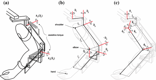
A popular form of support is an exoskeletal structure which enables assistance to be applied about individual joints. An example is the commercial ArmeoSpring (Hocoma AG) which provides adjustable force against gravity via two springs. Each joint is aligned in either the horizontal or vertical plane, as shown in Fig. 2.1a, with measured joint variables ![$$\varvec{ \varTheta } = [ \theta _1, \theta _2, \theta _3, \theta _4, \theta _5 ]^\top $$](/wp-content/uploads/2016/09/A352940_1_En_2_Chapter_IEq30.gif) . The patient’s arm is rigidly strapped to the exoskeleton support with lengths
. The patient’s arm is rigidly strapped to the exoskeleton support with lengths  ,
,  relating the shoulder joint to a fixed base frame.

![$$\varvec{ \varTheta } = [ \theta _1, \theta _2, \theta _3, \theta _4, \theta _5 ]^\top $$](/wp-content/uploads/2016/09/A352940_1_En_2_Chapter_IEq30.gif) . The patient’s arm is rigidly strapped to the exoskeleton support with lengths
. The patient’s arm is rigidly strapped to the exoskeleton support with lengths  ,
,  relating the shoulder joint to a fixed base frame.
Fig. 2.1
ArmeoSpring: a mechanical support, b kinematic relationships, and c human arm
Hence for the ArmeoSpring  and
and  are 5-by-5 inertial and Corelis matrices, and moments produced through gravity compensation provided by each spring yield the form
 ![$$\varvec{K}_a(\cdot ) = [0, 0, k_3(\theta _3), 0, k_5(\theta _5)]^\top $$](/wp-content/uploads/2016/09/A352940_1_En_2_Chapter_IEq35.gif) . Figure 2.1c shows the axes corresponding to anthropomorphic joints.
. Figure 2.1c shows the axes corresponding to anthropomorphic joints.

 and
and  are 5-by-5 inertial and Corelis matrices, and moments produced through gravity compensation provided by each spring yield the form
 ![$$\varvec{K}_a(\cdot ) = [0, 0, k_3(\theta _3), 0, k_5(\theta _5)]^\top $$](/wp-content/uploads/2016/09/A352940_1_En_2_Chapter_IEq35.gif) . Figure 2.1c shows the axes corresponding to anthropomorphic joints.
. Figure 2.1c shows the axes corresponding to anthropomorphic joints.
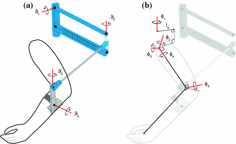
Fig. 2.2
SaeboMAS: a mechanical support and kinematic relationships, and b human arm
Another common structure is the end-effector type where support is only supplied at a single attachment point. An example is the SaeboMAS (Saebo, Charlotte, USA) shown in Fig. 2.2. Here the support takes the form ![$$\varvec{K}_a(\cdot ) = [k_1 (\theta _1), 0, 0, 0]^\top $$](/wp-content/uploads/2016/09/A352940_1_En_2_Chapter_IEq36.gif) .
.
![$$\varvec{K}_a(\cdot ) = [k_1 (\theta _1), 0, 0, 0]^\top $$](/wp-content/uploads/2016/09/A352940_1_En_2_Chapter_IEq36.gif) .
.2.1.4 Combined Dynamics
It is now assumed that within the necessary joint ranges there exists a unique bijective transformation between coordinate sets, given by  , which allows the mechanical support and human arm models to be combined. This explicitly holds for exoskeletal passive or robotic structures (where
  ), and can be extended to end-effector robot devices developed for rehabilitation. The Lagrangian equation in one variable can be expressed in terms of the other through application of the chain rule, and the results added to produce the combined model

where
 with
with  and
and  .
.
 , which allows the mechanical support and human arm models to be combined. This explicitly holds for exoskeletal passive or robotic structures (where
  ), and can be extended to end-effector robot devices developed for rehabilitation. The Lagrangian equation in one variable can be expressed in terms of the other through application of the chain rule, and the results added to produce the combined model
(2.6)

 and
and  .
.Now let each  be realized using continuous-time state-space model matrices
  ,
,  ,
,  (state, input and output respectively), with corresponding states
  . The system (2.6) can then be expressed over time interval
  in the following state-space form
![$$\begin{aligned} \dot{\varvec{x}}_s (t)&= \underbrace{ \left[ \begin{array}{c} \dot{\varvec{ \varPhi }}(t) \\ \varvec{B} ( \varvec{ \varPhi }(t))^{-1} \varvec{X} \big ( \varvec{ \varPhi }(t),\dot{\varvec{ \varPhi }}(t) \big ) \\ \varvec{M}_{A,1} \varvec{x}_{1} \\ \vdots \\ \varvec{M}_{A,m} \varvec{x}_{m} \end{array} \right] }_{ \varvec{f}_s \left( \varvec{x}_s(t) \right) } + \underbrace{ \left[ \begin{array}{c} \varvec{0} \\ \varvec{0} \\ \varvec{M}_{B,1} h_{{\textit{IRC}},1}( {u}_1(t) ) \\ \vdots \\ \varvec{M}_{B,m} h_{{\textit{IRC}},m}( {u}_m(t) ) \end{array} \right] }_{ \varvec{g}_s \left( \varvec{u}(t) \right) }, \nonumber \\ \varvec{ \varPhi }(t)&= \underbrace{ \left[ \begin{array}{cccc} \varvec{I}&\varvec{0}&\cdots&\varvec{0} \end{array} \right] \varvec{x}_s(t) }_{ \varvec{h}_s \left( \varvec{x}_s(t) \right) }, \quad \varvec{ \varPhi }(0) = \varvec{ \varPhi }_0, \end{aligned}$$](/wp-content/uploads/2016/09/A352940_1_En_2_Chapter_Equ7.gif)
where ![$$\varvec{x}_s(t) = [\varvec{ \varPhi }(t)^\top , \; \dot{\varvec{ \varPhi }}(t)^\top , \; \varvec{x}_{1}(t)^\top \; \cdots \; \varvec{x}_{m}(t)^\top ]^\top $$](/wp-content/uploads/2016/09/A352940_1_En_2_Chapter_IEq47.gif) , and the ith row of
, and the ith row of  is given by
![$$\begin{aligned} \varvec{X}_i \big ( \varvec{ \varPhi }(t),\dot{\varvec{ \varPhi }}(t) \big )&= \sum ^m_j \left( \varvec{M}_{C,j} \varvec{x}_{j}(t) F_{M,i,j} \big ( \varvec{ \varPhi }(t),\dot{\varvec{ \varPhi }}(t) \big ) \right) - \big ( \varvec{J}^\top ( \varvec{ \varPhi }(t) ) \big )_i \varvec{h}(t) \nonumber \\[-0.2cm]&\quad - \varvec{C}_i \big ( \varvec{ \varPhi }(t) ,\dot{ \varvec{ \varPhi } }(t) \big ) \dot{ \varvec{ \varPhi } }(t) - \varvec{F}_i \big ( \varvec{ \varPhi }(t) , \dot{ \varvec{ \varPhi } }(t) \big ) - \varvec{G}_i ( \varvec{ \varPhi }(t)) - \varvec{K}_i ( \varvec{ \varPhi }(t)).\nonumber \end{aligned}$$](/wp-content/uploads/2016/09/A352940_1_En_2_Chapter_Equ23.gif)
 be realized using continuous-time state-space model matrices
  ,
,  ,
,  (state, input and output respectively), with corresponding states
  . The system (2.6) can then be expressed over time interval
  in the following state-space form
![$$\begin{aligned} \dot{\varvec{x}}_s (t)&= \underbrace{ \left[ \begin{array}{c} \dot{\varvec{ \varPhi }}(t) \\ \varvec{B} ( \varvec{ \varPhi }(t))^{-1} \varvec{X} \big ( \varvec{ \varPhi }(t),\dot{\varvec{ \varPhi }}(t) \big ) \\ \varvec{M}_{A,1} \varvec{x}_{1} \\ \vdots \\ \varvec{M}_{A,m} \varvec{x}_{m} \end{array} \right] }_{ \varvec{f}_s \left( \varvec{x}_s(t) \right) } + \underbrace{ \left[ \begin{array}{c} \varvec{0} \\ \varvec{0} \\ \varvec{M}_{B,1} h_{{\textit{IRC}},1}( {u}_1(t) ) \\ \vdots \\ \varvec{M}_{B,m} h_{{\textit{IRC}},m}( {u}_m(t) ) \end{array} \right] }_{ \varvec{g}_s \left( \varvec{u}(t) \right) }, \nonumber \\ \varvec{ \varPhi }(t)&= \underbrace{ \left[ \begin{array}{cccc} \varvec{I}&\varvec{0}&\cdots&\varvec{0} \end{array} \right] \varvec{x}_s(t) }_{ \varvec{h}_s \left( \varvec{x}_s(t) \right) }, \quad \varvec{ \varPhi }(0) = \varvec{ \varPhi }_0, \end{aligned}$$](/wp-content/uploads/2016/09/A352940_1_En_2_Chapter_Equ7.gif)
(2.7)
![$$\varvec{x}_s(t) = [\varvec{ \varPhi }(t)^\top , \; \dot{\varvec{ \varPhi }}(t)^\top , \; \varvec{x}_{1}(t)^\top \; \cdots \; \varvec{x}_{m}(t)^\top ]^\top $$](/wp-content/uploads/2016/09/A352940_1_En_2_Chapter_IEq47.gif) , and the ith row of
, and the ith row of  is given by
![$$\begin{aligned} \varvec{X}_i \big ( \varvec{ \varPhi }(t),\dot{\varvec{ \varPhi }}(t) \big )&= \sum ^m_j \left( \varvec{M}_{C,j} \varvec{x}_{j}(t) F_{M,i,j} \big ( \varvec{ \varPhi }(t),\dot{\varvec{ \varPhi }}(t) \big ) \right) - \big ( \varvec{J}^\top ( \varvec{ \varPhi }(t) ) \big )_i \varvec{h}(t) \nonumber \\[-0.2cm]&\quad - \varvec{C}_i \big ( \varvec{ \varPhi }(t) ,\dot{ \varvec{ \varPhi } }(t) \big ) \dot{ \varvec{ \varPhi } }(t) - \varvec{F}_i \big ( \varvec{ \varPhi }(t) , \dot{ \varvec{ \varPhi } }(t) \big ) - \varvec{G}_i ( \varvec{ \varPhi }(t)) - \varvec{K}_i ( \varvec{ \varPhi }(t)).\nonumber \end{aligned}$$](/wp-content/uploads/2016/09/A352940_1_En_2_Chapter_Equ23.gif)
2.2 Model Identification
We next develop procedures to identify parameters in composite model (2.6) that can be used in a clinical setting. We first assume it is possible to manipulate each joint individually while measuring and recording the resulting joint angle and applied force signals. This is clearly not possible for all joints in the wrist and hand, and so alternative identification approaches for these structures are presented in Chap. 8.
Stay updated, free articles. Join our Telegram channel

Full access? Get Clinical Tree


