Kinematics of the Natural and Replaced Knee

Fig. 2.1

The joints of the human knee

This chapter discusses the historical and contemporary understanding of natural knee kinematics and the effect of total knee arthroplasty (TKA) on the kinematics of the joint. Initially, the issues associated with understanding the kinematics of a joint comprising three rigid bodies, which can each move in six degrees of freedom, will be discussed. The methods that have been used to assess knee kinematics will be highlighted and the issues involved in the analysis and interpretation of kinematic data considered. The main body of the chapter will then detail the historical development of the modern understanding of human knee kinematics, and finish with a discussion of the kinematics of the replaced joint.

Rigid Body Kinematics

The human knee comprises four bones: the tibia, the fibula, the femur and the patella; and two articulating joints: the tibiofemoral joint and the patellofemoral joint. The fibula provides no articulating surface at the knee joint and is, therefore, omitted from discussions of kinematics. Each of these bones, which are generally considered as rigid bodies, is free to move in six degrees of freedom: three rotations and three translations (Fig. 2.2). The knee is also constrained by a multitude of passive and active soft tissue structures. Most notable are the collateral and cruciate ligaments, and the extensor and flexor mechanisms [6]. Knee motion is governed by bone geometry and the soft tissue envelope. Assessing and describing the overall motion of the knee is, therefore, a complex task.

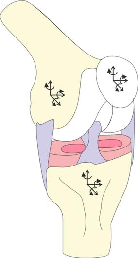
Fig. 2.2

Rigid body

The assessment of the motion of the bones within the knee, the kinematics, is normally considered individually for the two separate joints. This simplifies the situation to some extent, by limiting the problem to the description of the movement of one rigid body, e.g. the tibia, relative to a second rigid body, e.g. the femur.

The measurement of the movement of a rigid body can be a highly erroneous process. There are many methods to assess the movement of a rigid body, each with associated limitations. However, perhaps more significant, but less well understood, are the errors and uncertainties commonly introduced as a result of the methods used to combine, transform, and represent the kinematics of two bodies moving relative to one and other.

The methods used presently and historically to assess human knee kinematics are discussed in detail by Freeman and Pinskerova [7] and Pinskerova et al. [8], and summarised in this chapter. Before the advent of imaging techniques, such as X-rays, the movement of the bones within the knee joint was assessed through anatomical dissections of cadaveric samples [8]. Cadaveric bone samples were sliced and the shapes of the articulating surfaces assessed [9]. The influence of soft tissue structures has also been studied through sequential anatomical dissection of individual soft tissue structures [10–12]. These methods are destructive and invasive, and do not allow the assessment of the joint throughout the full range of motion [7].

As X-ray technology became more widely available and improved, surgeons and scientists were able to assess the joint articulating surfaces of both cadaveric and in vivo subjects in different static positions. However, X-rays only give a 2D view of what is a 3D joint and are generally taken in anatomic, but ultimately arbitrary, planes. They commonly led to a narrow and non-physiological view of knee motion, and the development of complex theories of motion which, although still prominent today, often led to an imperfect understanding of joint movement [8].

More recently, a variety of methods using a combination of X-rays, fluoroscopy, RSA, CT, MRI, and image matching methods have been developed to allow the assessment, in 3D, of the relative motions of the articulating surfaces, or the motion of the contact points between the bones during passive and active motions [7]. It is important to note that the relative motions of the articulating surfaces and the motion of the contact point between the bones are not equivalent measurements, and cannot be used interchangeably. An assessment of the relative motion of the articulating surfaces is usually achieved by tracking the displacement of the bones directly using anatomical reference landmarks and 3D image registration. An assessment of the motion of the contact point between two surfaces is achieved by tracking the point where the distance between the bone surfaces is smallest. This does not correspond to the motion of the bones [7]. It is also important to note the difference between a passive and an active situation. During an active kinematic assessment, when the muscles are loaded, the knee joint soft tissues will be under tension. The soft tissues will, therefore, guide and limit knee motion to a greater extent than during passive motion. This has been demonstrated to affect joint kinematics [13, 14].

Medical imaging techniques are often limited to static, quasi-static, or, at most, very controlled dynamic situations. Conversely, movement analysis methods can be used to assess joint kinematics during a wide variety of daily living activities. Markers located on the skin of the subject are tracked using optical sensors. A minimum of three non-orthogonal markers can be used to calculate the instantaneous position and attitude (rotational position) of a bone segment. Such calculations assume the segment is a rigid body and that minimal slip of skin and soft tissues occurred [15].

Mathematical methods, based on the model of the human body as a kinematic chain, comprising multiple links or bone segments, can then be used to estimate the kinematics of a joint, such as the knee. This estimation requires the reliable and consistent selection of a global reference system, repeatable anatomical landmark registration, and appropriate manipulation of position vectors and attitude matrices [16]. There are many ways to interpret position and attitude matrices: based on Cardan angles, helical axes, geometrical assumptions or anatomical locations [1, 17]. Some methods are at risk of gimbal-lock at certain degrees of flexion, and all of the methods are complicated by the coupled relationship between the different rotational degrees of freedom [17, 18]. Analysis has demonstrated that in degrees of freedom with relatively little motion, i.e. external/internal rotation of the knee, different methods can result in the calculation of angles which vary by more than 30° [17]. Issues associated with anatomical landmark registration and the discussion of whole joint kinematics in a consistent manner can also occur when imaging methods are used to assess joint motion. This complex subject is discussed in greater detail by Cappozzo et al. [17] and Woltring [18].

The assessment and description of the six degrees of freedom motion of rigid bodies, such as the bones within the knee, is complex, associated with a number of errors, and open to misinterpretation. These issues have to be borne in mind when assessing kinematic studies. However, as will be discussed in the following sections, consistent theories can be constructed, when the results of multiple studies are combined and compared in light of these limitations.

Normal Knee Kinematics¹

The kinematics of the human knee has been investigated for over 150 years (Fig. 2.3). The periods of development that lead up to the current understanding can be broadly split into three: early understanding, classical theory and modern theory (Fig. 2.3).

Fig. 2.3

Timeline depicting the development of the modern knee kinematic theories [2–4, 8, 19, 20]

Early Understanding

In 1836, the Weber brothers [9] dissected a human cadaver and examined the shapes and relative movements of the bones within various lower limb joints. They demonstrated the circular nature of the posterior femoral condyles, and that longitudinal rotation, around a medial pivot, occurs alongside flexion. Further early work, using an early form of motion capture systems, supported the assertion that the knee joint experiences longitudinal rotation coupled to any flexion movement [8].

The first radiographic study to be carried out on the knee led to the suggestion that it could be modelled as a linkage mechanism. Zuppinger assumed that the cruciate ligaments remain taut throughout the flexion range and, along with the tibia and femur, formed a rigid four bar linkage. Other early work disputed the assumption that the posterior cruciate ligament (PCL) was taut throughout the range of flexion. However, it was only the four bar linkage image that was remembered and incorporated into classical theory in the 1970s. Many of the other early studies, carried out largely by anatomists, were in German and largely forgotten as English became the primary language of science [8].

Classical Theory

Little work to develop understanding of knee joint kinematics was carried out in the period from 1917 to 1970. However, in the 1970s, scientists and engineers, mostly unaware of much of the early work published in German and French, began using X-rays and other imaging techniques to attempt to describe knee kinematics [8]. Sagittal plane X-rays were taken of cadaveric and in vivo knees. The axis of tibiofemoral flexion was assessed using the Rouleaux method, making the assumption that the two axes of the joint are planar. Such analyses, which are subject to significant errors if images are not taken in the plane of motion, demonstrated that the instantaneous centre of rotation of the knee, when viewed in the sagittal plane, moves in a semi-circle or a J shaped curve [2, 21–23]. The four bar linkage mechanism, originally proposed by Zuppinger and reprinted by Kapandji has classically been used to describe the complex motion inferred by the moving centre of rotation. This model was considered to describe not only flexion-extension of the knee joint, but also the femoral posterior translation and rotation known to occur with flexion. The four bar linkage mechanism does not take into account the axial rotation of the tibia relative to the femur previously reported to occur alongside flexion [2, 3].

Modern Theory

In the 1980s there was renewed interest in the anatomy of the distal femur, and how this may inform understanding of knee kinematics. Kurosawa et al. [4], used X-ray images and calliper measurements of cadaveric knees to demonstrate that the posterior femoral condyles can be modelled as spheres. The circularity of the distal femoral condyle was further demonstrated by Elias et al. [24], who indicated that the centre of the lateral and medial spheres corresponded with the insertion points of the collateral ligaments.

In 1993, Hollister et al. [20] demonstrated, using cadaveric specimens, that knee motion can be simply described as rotations around two non-orthogonal axes. These axes are not related to normal planes of motion and can, therefore, be difficult to interpret anatomically and surgically. Hollister was also able to demonstrate that the flexion axis, which coincides with the circular centres described by Elias et al. [24], does not move relative to the femur during the majority of the flexion range. The longitudinal axis of the knee passes though the medial plateau of the tibia and is not in the same plane as the flexion axis.

Using MRI scans Hollister also confirmed that, when viewed along the flexion axis, the posterior femoral condyles have a constant radius [20]. This work was taken further by Freeman, Eckhoff, and others [25–29], who demonstrated, using 3D imaging techniques such as MR, CT, and fluoroscopy, that the posterior section of the femoral condyles can be modelled as cylinders with coincident axes. This coincident axis is the flexion axis of the knee and does not correspond with the surgical transepicondylar axis [19].

The work of Hollister, Freeman, and others has led to the formulation of modern knee kinematic theory [1, 7, 20]. Modern theory is based around the notion that knee motion occurs in three distinct phases, as depicted by Fig. 2.4.

Fig. 2.4

Phases of knee motion (After: Freeman and Pinskerova [1])

The “Screwhome” arc of motion describes tibiofemoral flexion/extension from full extension to approximately 20° of flexion. In full extension both the collateral and cruciate ligaments are taut [12]. During a passive extension motion, at approximately 20° of flexion, the knee appears to rock as the femoral condyles shift from the flexion to the extension facets. The medial condyle rolls up on to the tibial extension facet causing its centre to move approximately 1.2 mm posteriorly, whereas the lateral condyle rolls down the tibial anterior horn moving up to 2 mm distally as the lateral collateral ligament (LCL) relaxes. This results in posterior roll back and a net internal tibial rotation, relative to the femur, in the order of 1° axial rotation for every 2° of flexion [1, 7, 12, 30, 31].

At, and near, full extension of the tibiofemoral joint, the patella is located proximal to the trochlear groove of the femur [32]. During this phase of motion, there is little femoral geometry to constrain the patella movement. It is, therefore, restricted largely by soft tissues, namely the retinaculum and quadriceps mechanism [33].

During the active flexion arc, approximately 20–120° of flexion, the femur rotates about the flexion axis [1, 7, 20]. During passive motion, in this range of flexion, the femoral medial condyle moves very little anterioposteriorly, whereas the lateral condyle moves posteriorly. This equates to a small amount of posterior roll back, and tibial internal rotation around a medial pivot of approximately 10–20° [1, 7, 13, 30, 34–37]. There are multiple theories as to the cause of this tibial rotation, which is reduced when muscle forces are present [13]. It has been suggested that tibial rotation may be a result of the lack of symmetry in the collateral ligaments; throughout flexion the medial collateral ligament (MCL) remains isometric, but the LCL slackens slightly with flexion [12, 38]. The posterior distal insertion point of the LCL also acts to force the lateral femoral condyle posteriorly and hence induce rotation [38]. Alternatively, it may be due to the difference in constraint and conformity provided by the lateral and medial menisci [1, 39].

Tibial rotation is undoubtedly necessary in deeper flexion to facilitate the femur and tibia moving in relation to each other [40]. However, its role in early flexion is less clear. Although tibial rotation is passively coupled to flexion, it can be reversed or prevented when muscle loading is applied, and may be an evolutionary hangover [7, 13, 28, 35, 40]. Posterior rollback in the natural knee is largely driven by the action of the cruciate ligaments and stabilised by the MCL [12, 41, 42].

During active flexion, the patella rotates around the femoral condyles with an axis of rotation that is parallel to the femoral flexion axis [43–47]. Patella flexion is proportional to tibiofemoral flexion but lags by approximately 30 % [48]. The patella contacts the trochlear groove at approximately 10–20° of femoral flexion [32, 33]. From this point until approximately 90° of tibiofemoral flexion, the patella runs deep within the congruent trochlear grove. Throughout this range of motion, femoral geometry forms the primary constraint to patella subluxation [33].

The patella initially translates medially and then laterally from approximately 30° of tibiofemoral flexion onwards (Fig. 2.5) [32, 43–45, 49–52]. With increased tibiofemoral flexion, the patella also rotates medially to a maximum of approximately 15° at 50° of tibiofemoral flexion [32]. This pattern is highly variable, even within the healthy population, and is greatly affected by foot orientation [43, 49, 53]. Similarly, the reported patterns of patella tilt vary widely. Many studies report a medial tilt in early tibiofemoral flexion, which becomes lateral from approximately 30° to 90° of tibiofemoral flexion [43, 49, 53]. Conversely, other studies have indicated an entirely lateral tilt, often demonstrating a medial lean in tibiofemoral deep flexion [43–45, 52, 54, 55]. The high variability in reported patella kinematics may be a result of the inherent instability in the joint, which is a result of limited bony constraints. However, the high variability may also be due to the wide range of assessment methods and the assumptions that have to be made when assessing bone kinematics [52, 53].

Fig. 2.5

Patella degrees of freedom

Tibiofemoral flexion in excess of approximately 120° is called passive flexion as the muscles have insufficient moment arms to actively move the limb. It is, therefore, only possible with additional external forces, such as body weight [1]. During the passive flexion arc of motion the tibia ceases to axially rotate and the femur as a whole begins to move posteriorly as the femoral condyles articulate with the tibial posterior horns [1]. There is some evidence that tibial rotation continues in Asian subjects [37]. During this range of motion the patella sits deeply within the intercondylar notch [56].

Knee Kinematics After Total Knee Arthroplasty

Early TKA designs aimed to facilitate load transfer at the knee via a planar hinge. Although still in use for patients with severe deformities and soft tissue insufficiencies, hinge designs have largely been replaced by total condylar designs. Total condylar implants replace both the tibial and femoral surfaces, and sometimes the patella articulating surface, with components that are not mechanically linked. Significant development has occurred in recent decades in terms of the design of the implants and the tools used to implant them [57].

The design of the femoral prosthetic component is not consistent across replacement systems [58]. Older implant systems are designed based on the traditional J curve or instantaneous centres of rotation theory of tibiofemoral kinematics. They, therefore, exhibit a range of sagittal radii in the functional range of motion and have been reported to suffer from mid-range instability as the collateral ligaments suddenly slacken when the centre of rotation changes [59, 60]. More recent designs are based on modern kinematic theory and only have one sagittal condylar radius in the functional range of motion. The centre of rotation of single radius knees is designed to coincide with the insertion points of the collateral ligaments. This maintains the natural ligament isometry in early and mid-flexion, preventing the issues of mid-range instability. Femoral component designs also vary in terms of frontal plane radii and trochlear groove design [61].

In the majority of commercially available designs, the tibial implant is split into base plate and bearing components to allow ease of manufacture, flexibility within surgery, and, if required, the ability to replace the bearing without requiring a full revision [62]. The bearing can be permanently locked to the base plate using wires or pins, in what is known as a fixed bearing configuration. Alternatively, it may be allowed to rotate and/or translate with respect to the tibial base plate. This is known as a mobile bearing [63]. Modern implant systems are supplied with a variety of bearings, which provide varying degrees of constraint to the tibiofemoral joint. The most common systems are defined as Cruciate Retaining (CR), Cruciate Sacrificing (CS) or Posterior Stabilised (PS).

Early CR designs were based on the retention of both cruciate ligaments and provided little tibial constraint. However, the retention of both cruciates added a significant amount of complexity to the procedure and prevented effective reconstruction of significant joint surface deformities. Most modern total condylar implants, therefore, require the removal of the anterior cruciate ligament (ACL) to enable placement of the prosthesis [64]. CR bearings have anterior cut outs to allow retention of the PCL, which is relied on to guide joint motion. The conformity, with respect to the femoral component, of CR bearings varies with manufacturer and model. Some designs use relatively shallow tibial plateaus and rely on the PCL to provide constraint, while others use conforming surfaces, which closely match the femoral geometry [58, 64, 65].

The retention of the PCL is thought to enhance the physiological relevance of the joint motion as it prevents anterior motion of the femur in the natural knee [12]. However, studies have indicated that the PCL may be unable to provide sufficient constraint without the ACL [66]. Some surgeons, therefore, routinely resect it. It may also be necessary to resect the PCL due to damage or degeneration. In these cases the surgeon may choose to use a CS or PS bearing. CS bearings are similar in design to CR bearings, but are all highly conforming [58], often with high anterior lips to prevent excessive anterior motion [63]. PS bearings have a cam-post system, which provides additional anterioposterior, but not mediolateral constraint, especially in deeper flexion [63]. The interaction of the post and cam guides the joint motion [65].

As Fig. 2.6 highlights, the percentage of patellae resurfaced during primary TKA procedures varies across the developed world [67–69]. Many papers and reports agree that the patellofemoral joint is one of the primary reasons for revision following TKA [70], but there is no consensus as to whether resurfacing is or is not beneficial [71]. Recent reviews and retrospective registry studies have highlighted the increased risk of failure in non-resurfaced joints but note the lack of reliable evidence to support or explain this, and disagree as to its significance [68, 72–76].

Fig. 2.6

Percentage of primary total condylar

There are a variety of patella implant designs used in modern TKA [77, 78]. The majority of implants are designed to sit on the surface of the cut bone, but some are intended to be inset into the bone. Most modern systems include a dome patella button option [79–86]. Some commonly used systems are also provided with asymmetric, medialised dome buttons [81, 84], or an anatomical, asymmetrical design [85]. Dome shaped designs are intended to be relatively forgiving to malplacement and soft tissue changes within the joint. Conversely, asymmetrical designs are intended to facilitate more anatomical and congruent tracking, and to increase the contact area within the patellofemoral joint [77].

Significant developments have taken place since early knee replacement designs were introduced in the 1970s. Despite this, as the following sub-sections will detail, in many ways modern TKA systems are not able to fully replicate natural tibiofemoral and patellofemoral kinematics.

Tibiofemoral Kinematics

Various in vivo and cadaveric studies have been carried out using motion analysis and fluoroscopic methods to assess the 3D kinematics of the tibiofemoral joint after TKA. There is limited evidence that some implant designs result in a reversal of the natural pattern of tibial internal rotation with knee flexion [50]. However, the majority of studies indicate that, following TKA, irrespective of design or constraint, tibial rotation is maintained, but significantly reduced [16, 34, 87–92]. In contrast, evidence suggests that tibial rotation is maintained at pre-surgery levels following uni-condylar knee replacement [91]. Uni-condylar knee replacement involves the resurfacing of only one set of femoral and tibial condylar surfaces. There is, therefore, no need to remove any soft tissue structures. The cruciate ligaments are able to continue to guide knee motion in a natural manner [12].

Only gold members can continue reading. Log In or Register to continue