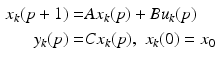
. Here the nonnegative integer k is the trial number and  denotes the number of samples on each trial, with the assumption of a constant sampling period. Suppose also that the dynamics of the system or process considered can be adequately modeled as linear and time-invariant. Then the state-space model of such a system in the ILC setting is
(2.1)
 is the state vector,
  is the output vector and
  is the control input vector.
In this model it is assumed that the initial state vector does not change from trial-to-trial. The case when this assumption is not valid has also been considered in the literature. The dynamics are assumed to be disturbance-free but again this assumption can be relaxed. It also possible to write the dynamics in input-output form involving the convolution operator or take the one-sided z transform and hence analysis and design in the frequency domain is possible. To apply the z transform it is necessary to assume  but in most cases the consequences of this requirement have no detrimental effects. For a more detailed analysis of cases where there are unwanted effects arising from this assumption, see the relevant references in Ahn et al. (2007), Bristow et al. (2006) and more recent work in Wallen et al. (2013).
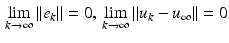
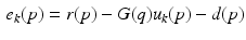
but in most cases the consequences of this requirement have no detrimental effects. For a more detailed analysis of cases where there are unwanted effects arising from this assumption, see the relevant references in Ahn et al. (2007), Bristow et al. (2006) and more recent work in Wallen et al. (2013).Let  denote the supplied reference vector. Then the error on trial k is
 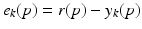 and the core requirement in ILC is to construct a sequence of input functions
 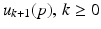 , such that the performance achieved is gradually improved with each successive trial and after a ‘sufficient’ number of these the current trial error is zero or within an acceptable tolerance. Mathematically this can be stated as a convergence condition on the input and error of the form
where  is termed the learned control and
  denotes an appropriate norm on the underlying function space. As one possibility, let
  denote the Euclidean norm of its argument and set
 ![$$||e|| = \max _{p \in [ 0, T]} ||e(p)||_{2}$$](/wp-content/uploads/2016/09/A306304_1_En_2_Chapter_IEq13.gif) . The reason for including the requirement on the control vector is to ensure that strong emphasis on reducing the trial-to-trial error does not come at the expense of unacceptable control signal demands. In application, only a finite number of trials will ever be completed but mathematically letting
. The reason for including the requirement on the control vector is to ensure that strong emphasis on reducing the trial-to-trial error does not come at the expense of unacceptable control signal demands. In application, only a finite number of trials will ever be completed but mathematically letting  is required in analysis of, e.g., trial-to-trial error convergence.
denote the supplied reference vector. Then the error on trial k is and the core requirement in ILC is to construct a sequence of input functions , such that the performance achieved is gradually improved with each successive trial and after a ‘sufficient’ number of these the current trial error is zero or within an acceptable tolerance. Mathematically this can be stated as a convergence condition on the input and error of the form(2.2)
is termed the learned control and denotes an appropriate norm on the underlying function space. As one possibility, let denote the Euclidean norm of its argument and set . The reason for including the requirement on the control vector is to ensure that strong emphasis on reducing the trial-to-trial error does not come at the expense of unacceptable control signal demands. In application, only a finite number of trials will ever be completed but mathematically letting is required in analysis of, e.g., trial-to-trial error convergence.The standard form of ILC algorithm or law computes the current trial input as the sum of the input used on the previous trial and a corrective term, i.e.,
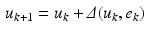
where  is the correction term and is a function of the error and input recorded over the previous trial. A large number of variations exist for computing the correction term, including laws that make use of information generated on a finite number (greater than unity) of previous trials. For the stroke rehabilitation application it is the repeated performance of a finite duration task (with the input on the current trial computed by adding a corrective term that is directly influenced by the previous trial error) that makes ILC particulary suitable.
(2.3)
is the correction term and is a function of the error and input recorded over the previous trial. A large number of variations exist for computing the correction term, including laws that make use of information generated on a finite number (greater than unity) of previous trials. For the stroke rehabilitation application it is the repeated performance of a finite duration task (with the input on the current trial computed by adding a corrective term that is directly influenced by the previous trial error) that makes ILC particulary suitable.An extensively used analysis and design setting for discrete systems is based on lifting in the ILC setting. Suppose that (2.1) is asymptotically stable and hence all eigenvalues of the state matrix A have modulus strictly less than unity. If this is not the case then a stabilizing feedback control loop must be first applied. For simplicity, consider single-input single-output (SISO) systems with an assumed relative degree of one, and hence in (2.1) the first Markov parameter  For the cases of multiple-input multiple-output (MIMO) systems and/or the assumption on the Markov parameter does not hold, refer to the relevant references in Ahn et al. (2007), Bristow et al. (2006).
For the cases of multiple-input multiple-output (MIMO) systems and/or the assumption on the Markov parameter does not hold, refer to the relevant references in Ahn et al. (2007), Bristow et al. (2006).Introduce
![$$\begin{aligned} y_{k} = \left[ \begin{array}{c} y_{k}(1)\\ y_{k}(2)\\ \vdots \\ y_{k}(T) \end{array} \right] ,\,\, u_{k} = \left[ \begin{array}{c} u_{k}(0)\\ u_{k}(1)\\ \vdots \\ u_{k}(T-1) \end{array} \right] ,\,\, d = \left[ \begin{array}{c} d(1)\\ d(2)\\ \vdots \\ d(T) \end{array} \right] . \end{aligned}$$](/wp-content/uploads/2016/09/A306304_1_En_2_Chapter_Equ4.gif)
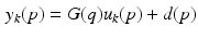
Then under the assumption that  , (2.1) can be written in the form

with
![$$\begin{aligned} G = \left[ \begin{array}{cccc} p_{1} &{} 0 &{} \ldots &{} 0\\ p_{2} &{} p_{1} &{} \ldots &{} 0\\ \vdots &{} \vdots &{} \ddots &{} \vdots \\ p_{T} &{} p_{T-1} &{} \ldots &{} p_{1} \end{array} \right] \end{aligned}$$](/wp-content/uploads/2016/09/A306304_1_En_2_Chapter_Equ6.gif)
where  and
and 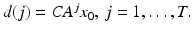
(2.4)
, (2.1) can be written in the form(2.5)
(2.6)
and 2.3.1 Control Laws and Structural/Performance Issues
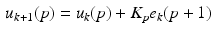
Consider the SISO version of the state-space model (2.1) and suppose that both the system dynamics and the measured output are deterministic, i.e., noise-free. Then a derivative, or D-type , ILC law constructs the current trial input as
![$$\begin{aligned} u_{k+1}(p) = u_{k}(p) + K_{d} [{e}_{k}(p + 1) - {e}_{k}(p)] \end{aligned}$$](/wp-content/uploads/2016/09/A306304_1_En_2_Chapter_Equ7.gif)
where  is a scalar to be designed such that
 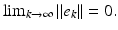 Also routine analysis shows that this condition holds if and only if
 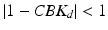 . Somewhat surprisingly, this condition is independent of the system dynamics embodied in state matrix A and can only be satisfied if
(2.7)
is a scalar to be designed such that Also routine analysis shows that this condition holds if and only if . Somewhat surprisingly, this condition is independent of the system dynamics embodied in state matrix A and can only be satisfied if The reason why trial-to-trial error convergence (k) is independent of the system state matrix is the finite trial length, over which duration even an unstable linear system can only produce a bounded output. In design based on a lifted model, the solution is to first design a stabilizing feedback control law for the unstable system and then apply ILC to the lifted version of the resulting controlled system. This step may also be required for stable systems to ensure acceptable transient dynamics along the trials. This results in a two stage design whereas the repetitive process, a class of 2D linear systems, setting allows simultaneous design for trial-to-trial error convergence and along the trial dynamics, see, e.g., Hladowski et al. (2010, 2012) where experimental verification on a gantry robot that replicates many industrial processes to which ILC is applicable is also given.
If the system model has relative degree greater than one it follows immediately that trial-to-trial error convergence cannot be achieved. This problem arises for many ILC laws and has received considerable attention in the literature, where one starting point is again the relevant references in the survey papers (Ahn et al. 2007; Bristow et al. 2006). This feature is also present in the 2D systems/repetitive process designs. The most that can be done for a system of relative degree h is to lose control over the first  samples along the trial and design a control law that gives convergence over the remaining samples.
samples along the trial and design a control law that gives convergence over the remaining samples.In ILC, once trial k is complete the following information is available for the computation of the control  : (1) Information from the entire time duration of any previous trial and (2) Information up to the current sample on trial
  . The following is one definition of causality in ILC.
: (1) Information from the entire time duration of any previous trial and (2) Information up to the current sample on trial . The following is one definition of causality in ILC.Definition 2.1
An ILC law is causal if and only if the value of the input  at time p on trial
  is computed only using data in the time interval [0, p] from the current and previous trials.
at time p on trial is computed only using data in the time interval [0, p] from the current and previous trials.For standard linear systems at sample instant p the use of information at future samples 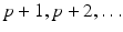 is non-causal and therefore any resulting control law cannot be implemented. The use of non-causal along the trial information in ILC laws is arguably the most important feature.
is non-causal and therefore any resulting control law cannot be implemented. The use of non-causal along the trial information in ILC laws is arguably the most important feature.Consider the ILC control laws
and
where the first is ILC non-causal and the second is causal. Also let q denote the forward time shift operator acting on, e.g., x(p) as  Then the dynamics of (2.1) can be written as
where  and this term can be extended to represent exogenous system disturbances that enter on trial k. Moreover, this disturbance term influences the error on trial k as
Hence the non-causal ILC law (2.8) anticipates the disturbance  and uses the input
  to preemptively compensate for its effects. This feature is not present in the causal ILC law (2.9).
(2.8)
(2.9)
Then the dynamics of (2.1) can be written as(2.10)
and this term can be extended to represent exogenous system disturbances that enter on trial k. Moreover, this disturbance term influences the error on trial k as(2.11)
and uses the input to preemptively compensate for its effects. This feature is not present in the causal ILC law (2.9).Causal ILC laws can be shown to be equivalent to a feedback control, i.e., an equivalent control action can be obtained directly from the ILC law and it has been asserted that causal ILC algorithms have little merit. See the discussion, with supporting references, in Bristow et al. (2006) that counters this argument but in any case the vast majority of implemented ILC laws are non-causal.
The finite trial length in ILC allows non-causal signal processing to be used. For many implementations, this is exploited in the form of zero-phase filtering of the previous trial error prior to the computation of the next trial input. An experimental example where zero-phase filtering is used is the gantry robot based results reported in Hladowski et al. (2010, 2012). Essentially, zero-phase filtering between trials can be used to remove unwanted effects, e.g., noise from the measured signals.
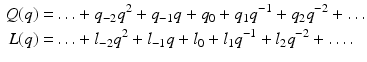
A commonly used ILC law is given by
![$$\begin{aligned} u_{k+1}(p) = Q(q) \left[ u_{k}(p) + L(q)e_{k}(p+1) \right] \end{aligned}$$](/wp-content/uploads/2016/09/A306304_1_En_2_Chapter_Equ12.gif)
where Q(q) is termed the Q-filter and L(q) is the learning function , but these designations are not universally used in the literature. The Q-filter and learning function L can be non-causal, in the ILC sense, with impulse responses
(2.12)