Fig. 19.1
This cut-through demonstrates a tear within the ACL (long arrow) on a 3D SPGR image (left) and a 2D Fast Spin Echo (FSE) T2 weighted image (right). The marrow is better visualized in the FSE image. Figure courtesy of Dr. Lorenzo Nardo, MD, UCSF
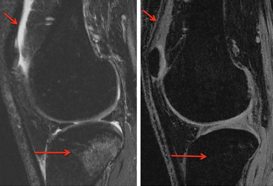
Fig. 19.2
Findings such as joint effusion and bone marrow edema are very common in acute injury and are noted in these images. On this cut-through of the lateral compartment of the knee, bone marrow edema (long arrow) and effusion in the joint (short arrow) are better seen on the 2D FSE T2-weighted sequence (on the left) than on 3D SPGR (on the right). However, on the SPGR image, the definition between bone and cartilage is better demonstrated. Figure courtesy of Dr. Lorenzo Nardo, MD, UCSF
A 3D version of the FSE sequence has recently been developed, featuring high contrast and isotropic spatial resolution; these developments have resulted in increased accuracy of cartilage imaging. The resulting image data can be reformatted for evaluation of the joint in various planes, and is comparable with multi-planar 2D FSE regarding the evaluation of cartilage, menisci, and ligament. One disadvantage of 3D FSE is that while it has aided the accuracy of cartilage imaging, imaging of the adjacent bone has not similarly improved [7, 8]. A variation of the 3D FSE sequence is 3D FSE SPACE, which varies the flip-angle of the applied pulses and provides high T2-weighted tissue contrast. The technique features better SNR and SNR efficiency (SNR normalized by time) compared to other sequences but is not as effective at delineating cartilage lesions as 2D FSE, has poor contrast between cartilage and fluid as well as between cartilage and surrounding tissues, and requires lengthy imaging times [9–11].
Three-dimensional spoiled-gradient-recalled acquisition in steady state (3D SPGR) features higher sensitivity than 2D techniques and is comparable to arthroscopy in the depiction of cartilage defects [12, 13]. The sequence elevates the signal intensity of cartilage versus other tissues and features nearly isotropic spatial resolution. However, the elevated cartilage signal results in poor cartilage-to-fluid contrast, so small defects and edema can be overlooked [11]. In addition, 3D SPGR is unreliable for assessment of joint anatomy aside from cartilage, and long acquisition times are necessary (Figs. 19.1 and 19.2). These sequences have been primarily used for cartilage volume and thickness quantification [14].
Like 3D SPGR, 3D dual-echo steady-state (DESS) imaging is a gradient-recalled echo (GRE) sequence with acquisition in a steady state. In some regards, DESS is superior to SPGR, as DESS features a higher SNR as well as greater cartilage-to-fluid distinction than does SPGR. The quality of DESS in cartilage evaluation is comparable to that of other GRE sequences; 3D DESS showed comparable diagnostic accuracy and precision, and can assess cartilage thickness, volume, and longitudinal change in cartilage thickness similarly to other GRE sequences (Fig. 19.3) [15, 16].
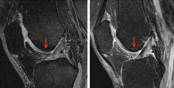
Fig. 19.3
Comparison between 3D sagittal dual-echo steady-state (DESS, left) and T2-weighted (right) images at the level of the ACL. The cartilage is well-demonstrated on the DESS image, while on the T2-weighted image, the presence of chemical shift artifacts makes the correct visualization of the cartilage difficult, especially on the femoral aspect (arrow). Figure courtesy of Dr. Lorenzo Nardo, MD, UCSF
Balanced steady-state free precession (3D bSSFP) imaging also provides good cartilage-to-fluid contrast; this is achieved by selectively increasing the signal of fluid without altering the cartilage signal. For diagnosing cartilage morphology, 3D bSSFP is comparable to 2D sequences and other 3D GRE sequences; however, 3D bSSFP can also effectively image other anatomical features in the knee such as ligaments and menisci [17–19].
Like 3D bSSFP, 3D driven-equilibrium Fourier transform (DEFT) imaging achieves cartilage-to-fluid distinction by selectively elevating the fluid signal. The 3D DEFT sequence does so with an applied 90° pulse, which results in a higher signal from anatomical features with long T1 relaxation time, such as fluid. The effectiveness of 3D DEFT in the diagnosis of cartilage lesions has been shown to be similar to 2D techniques as well as SPGR [11, 20]. The disadvantages of the 3D DEFT sequence include long acquisition time, low sensitivity to bone marrow abnormalities, and elevated fat signal due to inadequate lipid suppression.
The longest-established rubric for osteoarthritis (OA) image grading is the Kellgren–Lawrence (KL) scale, which assigns a score based on the severity of degeneration as seen on an X-ray image [21]. The KL grading system provides a simple, low-cost assessment of structural change based on joint space narrowing and osteophytes, both readily identifiable OA hallmarks. A number of studies have also used KL grading to evaluate longitudinal OA progression [22, 23].
By the early 1990s, as MRI revealed its potential to provide insight into OA, an alternate MRI-based approach to OA assessment and diagnosis emerged alongside the X-ray image and KL grading. Spector and Cooper commented on inconsistencies in the descriptions of radiographic features by Kellgren and Lawrence themselves as well as inconsistencies between grading at different joints; they also raised concerns about the associations of osteophyte formation with low KL grade and joint space narrowing (JSN) with high grade [24]. Since osteophyte formation and JSN are caused by independent processes, the KL scale provides a skewed depiction of OA progression [25]. The KL system does not evaluate the patellofemoral joint, nor can it assess tissues not visible on radiographs such as cartilage, ligaments, menisci, or the joint capsule [26–28].
While the KL system assigned a single score to the whole joint, the alternative approach favored separate assessment of bone and soft tissue [29]. The emerging technique initially borrowed grading scales used in arthroscopy [30]. Since then, four compartment-based, semiquantitative systems have been formulated to evaluate MR images of cartilage: the Whole-Organ Magnetic Resonance Imaging Score (WORMS) system was the first. WORMS grading assigns separate scores not only to the various knee cartilage compartments (Fig. 19.4), but also bone, menisci, and ligaments. The system also assesses joint effusion, loose bodies, and periarticular cysts [31].
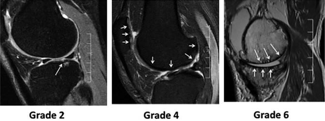
Fig. 19.4
Representative MR images with different stages of cartilage lesions and corresponding WORMS scores
Like WORMS, the Knee Osteoarthritis Scoring System (KOSS) evaluates cartilage, bone, and menisci, and records the presence and extent of effusion, synovitis, and cysts. KOSS also demonstrated both high inter-observer and intra-observer reproducibility; WORMS made no mention of intra-observer reproducibility [32]. The Boston-Leeds Osteoarthritis Knee Score (BLOKS), assesses the same features as WORMS and KOSS, but describes bone marrow edema-like lesions (BMEL) in further detail [33]. The MRI Osteoarthritis Knee Score (MOAKS) system further refines the rubrics of previous scoring instruments, particularly BLOKS. MOAKS features an altered BMEL scoring method, adds scoring for cartilage subregions, and incorporates additional categories of meniscus pathology [34].
The Magnetic Resonance Observation of Cartilage Repair Tissue (MOCART) system was specifically intended to evaluate repair cartilage following surgical interventions such as microfracture, chondrocyte transplantation, or osteochondral transplantation [35]. MOCART showed a strong, significant correlation with clinical outcome [36], and the MOCART system remained effective for both 2D and 3D imaging techniques [37]. The greatest limitation of MOCART is that it only evaluates the repair site, ignoring the remainder of the joint. To simultaneously assess change in cartilage repair sites and the surrounding native anatomy, the Cartilage Repair Osteoarthritis Knee Score (CROAKS) combined variables from MOCART and MOAKS in a comprehensive system suitable for whole-joint grading [38].
Quantitative morphological measures of other features such as bone marrow edema like lesions, meniscal injuries and fractures after anterior cruciate ligament injury have also been quantified, and have been associated with long term evolution into OA. Frobell et al. [39] found fractures in 60 % of ACL injured knees. Meniscal tears were found in 36 % subjects in one compartment, in 20 % of subjects extended to two compartments. BMEL are a common manifestation (98 % of subjects), especially in the lateral compartment (97 %). These authors also demonstrated that 1 year after injury joint fluid and BMEL volume decrease gradually; however, BMEL still persisted and cartilage volume showed increases in certain femoral compartments and decreases in others [40].
Quantitative Imaging of Cartilage Post-injury
Imaging T2 Relaxation Time
The basic premise of MRI is the excitation of protons and their subsequent relaxation back to an equilibrium state; the T2 MRI sequence evaluates the excitation–relaxation phenomenon of water protons with regard to the surrounding proteins. T2 refers to the spin–spin relaxation time, related to the rate at which nuclei lose phase coherence following excitation. Nuclei in phase coherence after excitation result in transverse magnetization and a strong MR signal. When nuclei lose phase coherence, the signal diminishes.
Cartilage is primarily composed of water and proteins such as type-II collagen and proteoglycans (PG). Water protons surrounded by the cartilage matrix undergo interactions with the various macromolecules, which cause faster magnetization decay and a shorter T2. Free water, however, experiences fewer of these interactions, lengthening T2. Differences in T2 are thus sensitive to variations in the free water content of cartilage [11, 41–44]. Studies have demonstrated that cartilage T2 is correlated with water content [45] but poorly with PG content [46]. Xia et al. showed using microscopic resolutions, that spatial variation in T2 is dominated by the ultrastructure of collagen fibrils, and thus angular dependency of T2 with respect to the external magnetic field can provide specific information about the collagen structure [30]. This angular dependency of T2, however, also results in the “magic angle” effect and commonly seen laminar appearance in cartilage imaging [47, 48]. Using clinically relevant resolutions, T2 studies revealed three laminae in cartilage – a deep layer adjacent to the bone, a superficial layer on the articular surface, and a transitional layer in between [49]. T2 generally increases across cartilage from the bone layer to the articular layer [50, 51]. Histologic experiments related regional T2 variation to differences in collagen orientation and distribution from one layer to the next.
Thus, collagen degradation as seen in osteoarthritis allows increased movement of free water and T2 has been shown to be elevated in patients with osteoarthritis [48, 52, 53] (Fig. 19.5). Studies using grey level co-occurrence matrix (GLCM) texture analysis of cartilage have shown that T2 is also more heterogeneous in osteoarthritic cartilage than in controls [53]. Though some studies have found associations between T2 and osteoarthritis in patellar cartilage [54], tibiofemoral cartilage has been the more noteworthy region for osteoarthritic change [48]; the vast majority of studies investigating T2 and osteoarthritis report significant findings in tibiofemoral cartilage. This is most likely due to the weight-bearing role that the tibiofemoral compartment plays in normal daily function and movement. T2 has shown a strong, significant correlation with a collagen degradation serum biomarker and a significant negative correlation with concentration of glycosaminoglycans (GAG), the component chains of proteoglycans [55], albeit with considerably small sample size.
Fig. 19.5
T1ρ and T2 maps of a healthy control (a), a subject with mild OA (b) and a subject with severe OA (c). Significant elevation of T1ρ and T2 values were observed in subjects with OA. T1ρ and T2 elevation had different spatial distribution and may provide complementary information associated with the cartilage degeneration
T2 elevation has also been associated with trabecular bone loss [56] and BMEL [54], a common occurrence in ACL injury and traumatic injury, and T2 GLCM heterogeneity has been associated with both BMEL and meniscal lesions [53]. T2 also has some degree of predictive power regarding osteoarthritis. In a cohort with KL and WOMAC pain scores of 0, those determined “at risk” for osteoarthritis had significantly elevated and heterogeneous cartilage T2 [57]. In addition, T2 at baseline is associated with progression of osteoarthritis and cartilage defects 2–3 years later [54, 58]. In subjects with ACL injury, 1 and 2 years post-reconstruction, T2 values in cartilage of the central aspect of the medial femoral condyle were significantly elevated compared with control knees, indicating a potential change in cartilage biochemistry akin to OA [59].
Finally, T2 has been used to distinguish repair cartilage from normal cartilage; in an equine model, control cartilage showed the expected trend of T2 spatial distribution, but sites of cartilage autograft harvest as well as microfracture sites did not [60]. A multimodal approach using T2, diffusion weighted imaging and grading of MR images has been used for assessing post-operative cartilage. While grading did not show differences between the two repair techniques, T2-mapping showed lower T2 values after microfracture, and diffusion weighted imaging between healthy cartilage and cartilage repair tissue in both procedures [61]. Mamisch et al. [62] prospectively used T2 cartilage maps to study the effect of unloading during the MR scan in the postoperative follow-up of patients after matrix-associated autologous chondrocyte transplantation (MACT) of the knee joint. They demonstrated that T2 values change with the time of unloading during the MR scan, and this difference was more pronounced in repair tissue. The difference between the repair and control tissue was also greater after longer unloading times, implying that assessment of cartilage repair is affected by the timing of the image acquisition relative to unloading the joint.
Articular cartilage has very limited intrinsic regenerative capacity, making cell-based therapy a possible approach for cartilage repair. Tissue engineered collagen matrix seeded with autogenous chondrocytes designed for the repair of hyaline articular cartilage have also been proposed and early studies combining MR grading and quantitative T2 mapping have been used to assess the impact of such repair [63]. In addition to fill efficacy the layered appearance or partial stratification of T2 as a result of collagen orientation was detected in this study for two patients at 12 months and four patients at 24 months.
Imaging T1ρ (rho) Relaxation Time
A similar sequence that has recently gained widespread use is T1ρ (T1 rho) or spin-lattice relaxation in the rotating frame. The sequence employs a constant, low-power radiofrequency (RF) pulse known as a “spin-lock” in the transverse plane [11, 41, 43, 44], which eliminates T2 relaxation. As is the case for T2, T1ρ relaxation is affected when water interacts with large macromolecules. In vitro studies have showed that the elevation of T1ρ relaxation time was correlated with PG loss in both bovine [46, 64] and human cartilage [65], and with histological grading [65, 66]. In T1ρ quantification experiments, the spin-lock techniques reduce dipolar interactions and therefore reduce the dependence of the relaxation time constant on collagen fiber orientation [67]. This enables more sensitive and specific detection of changes in PG content using T1ρ quantification, although T1ρ changes in cartilage may be affected by hydration and collagen structure as well. Early experiments with the T1ρ sequence found a similar but not identical spatial distribution to that of T2, with a trend of increase across the cartilage from bone layer to articular layer [68, 69]. Increases in mean T1ρ and T1ρ GLCM heterogeneity are associated with OA [66, 70, 71]. Studies have also shown significant T1ρ increase in more severe OA as compared to milder OA (Fig. 19.5), controls, or both [72, 73]. Cartilage T1ρ elevation has also been associated with trabecular bone loss [56], presence and location of BMEL [74], and higher WOMAC scores [75, 76]. In addition, elevated baseline T1ρ has been shown to predict OA progression at 2-year follow-up [58].
While T2 changes have been associated with collagen concentration and arrangement, biochemical assays suggest that T1ρ is more sensitive to proteoglycan content than to collagen [65, 77] and show that elevated T1ρ is associated with proteoglycan loss [64, 65, 78, 79]. Comparisons between T1ρ and T2 have found that T1ρ features superior delineation of cartilage lesions [80], signal-to-noise ratio [80], larger range [70], higher effect size [70], and greater percentage change with increasing severity of osteoarthritis [66] as compared to T2.
In patients with acute ACL tears, significantly increased T1ρ values were found at baseline (after injury but prior to ACL reconstruction) in cartilage overlying BMEL when compared with surrounding cartilage at the lateral tibia [56, 81]. In the posterolateral tibial cartilage, T1ρ values were not fully recovered 2 after ACL reconstruction. T1ρ values of medial tibiofemoral cartilage in ACL-injured knees increased over the 2-year study and were significantly elevated compared to that of the control knees (Fig. 19.6). Concomitant meniscal injury also reflected changes in articular cartilage, patients with lesions in the posterior horn of the medial meniscus exhibited significantly higher T1ρ values in weight-bearing regions of the tibiofemoral cartilage than that of control subjects over the 2-year period, whereas patients without medial meniscal tears did not [59].
Fig. 19.6
T1ρ Maps of ACL-injured knees
Using arthroscopy as a gold standard, Nishioka et al. have shown that in anterior cruciate ligament injured knees, authors have demonstrated that T1ρ has a sensitivity and specificity of 91.2 and 89.5 % respectively for detecting grade 1 cartilage lesions (as assessed by the ICRS grading system). On the other hand, the sensitivity and specificity for T2 were 76.5 and 81.6 %, respectively [82]. The cutoff values for determining the presence of a cartilage injury were determined using ROC curves to be 41.6 and 41.2 for T1ρ and T2 respectively.
A combined T1ρ and T2 study examining repaired and the surrounding cartilage has demonstrated differences in cartilage after micro-fracture and mosaicplasty 3–6 months and after a year [83] (Fig. 19.7). In subjects who had micro-fracture for focal cartilage defects, primarily in the medial femoral condyle, Theologis et al. found that while the average surface area of the lesions did not differ significantly overtime, at 3–6 months, repaired tissue had significantly higher full thickness T1ρ and T2 values relative to surrounding cartilage [84]. After 1 year, this significant difference was only observed for T1ρ values. Analysis of the different laminae of cartilage also showed different trends, with the superficial layer having significantly higher T1ρ value after 12 months, while the T2 values had reached the levels of the normal cartilage. Thus, these methods may be used to probe the level of integration of the repair tissue over time [83].
Fig. 19.7
Representative T1ρ maps of repaired tissue (RT) and normal cartilage (NC) divided into deep and superficial layers (black line) 3–6 months and 12 months after microfracture (left) and mosaicplasty (right) surgeries. The superficial and deep layers of RT 3–6 months after microfracture have elevated T1ρ values compared to NC. After 1 year, the RT is more homogeneous. The superficial layer of RT 3–6 months after mosaicplasty has elevated T1ρ values relative to NC. The deep layer is similar to NC. After 1 year, deep and superficial layers of RT resemble those of NC
Delayed Gadolinium-Enhanced MRI of Cartilage (dGEMRIC)
The main premise of dGEMRIC is derived from variations in fixed-charge density (FCD) of cartilage [11, 41–44, 85]. Proteoglycan content is thought to influence cartilage FCD, as proteoglycans have glycosaminoglycan (GAG) side chains rich with negatively charged carboxyl and sulfate groups. Ions in the cartilage matrix will distribute accordingly in relation to the FCD and approximate the GAG concentration and distribution. Cations will pool in areas of high FCD; anions, in areas of low FCD. The ionic compound gadopentetate dimeglumine, or Gd(DTPA)2−, is an effective and FDA-approved contrast medium for use in human MRI. The highly paramagnetic Gd(DTPA)2− reduce the T1 relaxation time of surrounding tissue, such that areas of high Gd(DTPA)2− concentration will result in reduced relaxation time, and areas of low Gd(DTPA)2− will have elevated relaxation time. Since Gd(DTPA)2− is an anion, it will accumulate in cartilage regions with low FCD and, by extension, low GAG concentration.
Cartilage lesions in specimen studies were first revealed by signal intensity differences between cartilage and contrast medium [86]; since then, lesions been revealed quantitatively by lowered T1 + Gd(DTPA)2− values [87, 88], even focal lesions surrounded by largely intact cartilage [68]. Biochemical studies have found a positive correlation between T1 + Gd(DTPA)2− and GAG concentration [88, 89], and between in vitro and in vivo T1 + Gd(DTPA)2− values [89]. In imaging studies, T1 + Gd(DTPA)2− has been shown to be significantly elevated in controls versus osteoarthritic individuals, and in moderate osteoarthritis versus severe cases [90, 91]. Finally, dGEMRIC has shown a strong correlation with WOMAC pain scores [92].
Fleming et al. have shown a significant difference (13 %) in the mean dGEMRIC indices of the medial compartment between ACL injured and uninjured knees (P < 0.007) [93]. Despite its strengths, dGEMRIC is an invasive and time-consuming procedure. The quickest delivery of Gd(DTPA)2− into cartilage is intravenous administration [87], and the joint of interest must be moved for 10 min afterward to distribute the contrast medium [94]. Data acquisition also begins 90 min post-injection [95].
Sodium Imaging
Sodium MRI imaging provides a noninvasive protocol specific to proteoglycan assessment. Sodium-23 is an ideal MRI contrast agent, occurring naturally in the body and possessing a nuclear spin momentum [11] due to its odd number of protons. Cations like Na+ will pool in areas of high negative FCD; since negatively charged proteoglycans influence FCD, Na+ concentration will be elevated with high proteoglycan content. Reduction in Na+ MRI signal has been correlated to proteoglycan depletion through FCD mapping [79] and trypsinization assays [96, 97]. Na+ MRI has shown a significant increase of Na+ T1 and Na+ T2 in proteoglycan-depleted cartilage [98]; Na+ relaxation times follow the same trend as proton relaxation times in compromised cartilage. Finally, the SNR of Na+ MRI is significantly higher for native cartilage than for repair tissue [99, 100]. There are a number of difficulties with Na+ MRI; Na+ ions exist in the body at lower concentrations than do H+ ions, and Na+ features a lower resonant frequency and shorter T2 relaxation time. These factors necessitate high magnetic field strength, special equipment, and lengthy imaging to attain a proper SNR [11, 44].
Glycosaminoglycan Chemical Exchange-Dependent Saturation Transfer (gagCEST)
Sodium MRI and dGEMRIC both use FCD to indirectly measure proteoglycan content in cartilage. Glycosaminoglycan chemical exchange-dependent saturation transfer (gagCEST) aims to directly measure proteoglycans by observing the behavior of −OH protons in GAG [101]. An off-resonance pulse targets restricted protons such as those bound to a macromolecule; the pulse excites and saturates these protons in the process [41, 43]. The excited, saturated protons then exchange magnetization with surrounding free water molecules. Free water protons lose magnetization more slowly than do restricted protons; however, since restricted proton magnetization is more rapidly dephased, water molecules receiving magnetization from restricted protons experience faster dephasing and lower signal. gagCEST involves the transfer of the excited −OH protons themselves, present throughout cartilage GAG. The contrast achieved is quantified as CEST effect or CEST asymmetry. In regions of low GAG content, low transfer occurs, and lower signal is observed.
CEST signal decreases with increased ex vivo proteoglycan depletion by trypsinization, as well as cartilage lesions in vivo [101]. gagCEST has shown useful results when evaluating repair cartilage following microfracture and chondrocyte transplantation [99, 100]. Asymmetry is significantly higher in native versus repair cartilage, and locations of gagCEST signal reduction agreed with those found with Na− MRI. The ratio of native to repair cartilage determined by gagCEST also negatively correlated with MOCART score [99].
Image quality is adversely affected by variations of the principal magnetic field (B0) within cartilage, low signal, and interference due to magnetization transfer from water and other macromolecules. The gagCEST signal has shown improvement with B0 correction [102], imaging at 7T instead of 3T [102], and a uniform magnetization transfer (uMT) technique that has effectively eliminated extraneous magnetization transfer effects [103].
Diffusion-Weighted Imaging (DWI)
Diffusion-weighted imaging (DWI) measures the motion of free water in cartilage. In DWI, two diffusion-sensitizing gradient pulses are applied; the first dephases the spins of molecules in the tissue, and the second rephases the spins. Only the spins of stationary molecules will be fully rephased by the second pulse; the spins of mobile molecules such as free water will not refocus and thus result in MR signal loss [11, 42, 43].
With DWI, one can measure the apparent diffusion coefficient (ADC) of free water, with a higher ADC indicating increased diffusion capability. Low ADC is indicative of slower diffusion and healthy cartilage, as the protein matrix serves as a barrier to free water movement [47]. An early study of diffusion MRI revealed that the diffusivity of several ions and water decreased in cartilage as compared to free solution [104]. Water diffusivity is elevated in proteoglycan-depleted cartilage [104, 105]. In addition, the diffusion coefficient is higher in repair cartilage following chondrocyte transplantation versus controls at early and late follow-up time points; DWI can still distinguish between repair and native cartilage 4–5 years post-transplantation [37, 106]. Additional results suggest that DWI has the capability to monitor the maturity of repair cartilage [37], and that it detects increased heterogeneity in repair versus native cartilage [106].
Periarticular Implants and Imaging
Unfortunately, post traumatic arthritis cannot be prevented and there is no effective treatment currently available. Low impact exercises, strengthening muscle around the joint and pain management can improve the quality of life of patients significantly. These measures help in alleviating the condition but cannot cure the arthritis. In some advanced cases, metallic implants may be used to surgically reconstruct the whole joint or a part of it. According to the Center for Disease Control and Prevention (CDC), there have been 719,000 total knee and 332,000 hip replacements in the USA in 2010 [107]. Joint replacement metallic parts are normally made of titanium, cobalt-chromium, or MR-safe stainless steel (screws), which are non-ferromagnetic and are convenient for MR imaging.
Standard MR sequences are used post operatively to look at the success of implantation, identify potential complications and to look at cartilage healing status. Although any imaging technique discussed in the first part of this chapter may be used to investigate the post operative changes, the presence of these implanted metal objects cause problems and produce artifacts near the implants interfering with the clinical quality of the MR images (Fig. 19.8). Although implants made of ceramic with even lower magnetic properties, longer lasting and higher biocompatibility (http://www.hss.edu/newsroom_11290.asp) compared to the ones currently being used have been developed, they have not been accepted widely by the orthopedic surgeons [108]. This part of the chapter discusses the artifacts, their causation factors, pulse sequences that are used to minimize these artifacts and emerging artifact reduction techniques.
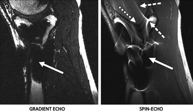
Fig. 19.8
Examples of artifacts observed in MR images due to presence of stainless steel screws in healthy 37-year-old man. Left: In gradient-echo image with ±62.5 kHz receive bandwidth. Right: spin-echo image with ± 16 kHz receive bandwidth. Solid arrows show signal loss that can be due to dephasing or from signal being shifted away from region. Dotted arrow in B shows geometric distortion of femoral condyle, and dashed arrows show signal pile-up, which can be combination of in-plane and through-slice displacement of signal from multiple locations to one location. Reprinted with Permission from ARRS
Artifacts near metal implants can be broadly categorized into in-plane and through-slice artifacts. The most common in-plane artifacts related to metal implants occur in the readout direction and cause signal voids due to dephasing, failure in fat suppression techniques, signal pile-up, or geometric distortions near the implants. Through-slice artifacts are commonly seen in the form of slice distortion in the excited slice [109, 110].
Signal voids occur due to the fact that there is no MRI signal from metal. Other artifacts like geometric distortions and signal pile-up occur because of metal induced magnetic field variations that result in a phenomenon known as “susceptibility” variations between the metal and the surrounding tissue. Magnetic susceptibility (“χ”) is defined by the magnitude of a material’s response to a magnetic field. When an object is placed in a magnet with homogenous magnetic field, the object depending on its susceptibility interferes with the imaging gradient field [111]. The material’s magnetization is equal to the dimensionless susceptibility “χ” multiplied by the applied magnetic field strength (B0). As seen in Table 19.1, the susceptibility of metals used in implants is much higher than the surrounding tissue. The tissue–air interface by itself is also capable of producing susceptibility artifacts that are noticeable on MR images. These susceptibility differences give rise to inhomogeneities in the local magnetic field. These field variations are affected by various factors as seen in Table 19.2, which describes general factors affecting metal implant artifacts.
Material | Susceptibility (χ, ppm) |
Human tissue | −10 |
Air | 0.36 |
Titanium | 178 |
Cobalt-chromium | 900 |
Stainless steel (MR safe) | 3,000–7,000 |
Factor | Effect |
Metallic composition of the implant | Non-ferromagnetic implants (titanium alloy) produce less artifacts than ferromagnetic (stainless steel) |
Implant size | Smaller implants produce less artifacts than larger |
Orientation of the implant | Artifact size increases and shape varies with increase in angle between the implant and the direction of the main magnetic field |
Magnetic field strength | Lower field strength produce less artifacts than higher field strength magnets |
Pulse sequence | Signal loss due to implants in Spin echo (SE) based sequences less compared to Gradient echo (GRE) sequences |
Pulse sequence parameters | Smaller voxel size, high resolution matrix, longer echo train length, shorter TEs and thinner slices produce less artifacts |
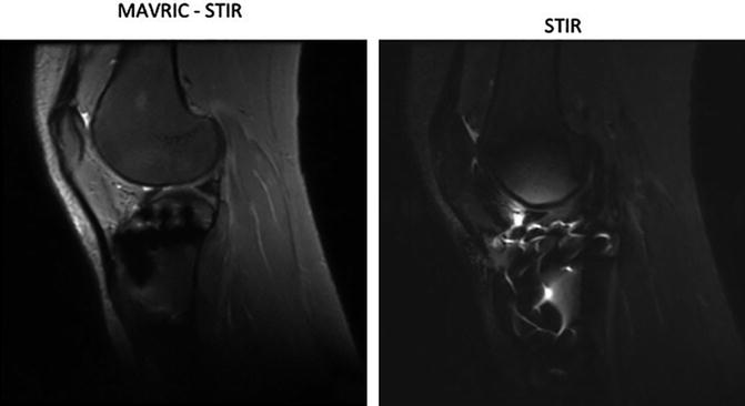
Apart from the signal loss and geometric distortions an important impediment to imaging near metal are the artifacts caused by failure of fat suppression and signal pile up. The suppression of fat signal is very useful to improve the soft tissue contrast in anatomical MR images. The bright (hyper-intense) appearance of fat causes problems in contrast enhanced bright lesions in T1 weighted images. Likewise, in T2 weighted images, the bright fat tissue signal intensity is confused with fluid or lesions exhibiting similar signal intensity. Also, being the second most abundant after water protons in the human body, fat protons are the major contributor of chemical shift artifacts. The most common technique used to avoid these artifacts is chemically selective fat suppression, also called fat saturation. This technique selectively excites fat instead of water molecules taking advantage of the fact that the resonant frequency of fat is ~220 Hz below water at 1.5T. However, the frequency difference (in the 3–80 kHz range) near metallic implants are much greater than the chemical shift frequency, which causes the fat saturation pulse to miss the resonant frequency of fat near metal implants altogether [108, 112]. Currently, the standard methods used for fat suppression in imaging near metal are STIR (Short T1 Inversion Recovery) [113] and Dixon method [114]. The T1 relaxation time of fat at 1.5T is ~230 ms, which is shorter than most of the other tissues in the body. This property is exploited in STIR, by using a short inversion time to null the signal from fat while maintaining the signal from water and soft tissue (Fig. 19.9). A 180° RF pulse is applied that inverts the magnetization followed by a 90° RF pulse which brings the residual longitudinal magnetization in the transverse plane where it is read by the RF coils. The delay between the 180 and 90° pulses is called inversion time (TI). In simple terms, in DIXON (2-point) method, two images are acquired, one when the water and fat is in-phase and the second in which water and fat is out of phase. During reconstruction a water only image can be calculated. The “point” refers to the number of images acquired [115].
 Arthritis That Develops After Joint Injury: Is It Post-Traumatic Arthritis or Post-Traumatic Osteoarthritis?
Post-Traumatic Arthritis: Definitions and Burden of Disease
Potential Targets for Pharmacologic Therapies for Prevention of PTA
Arthritis That Develops After Joint Injury: Is It Post-Traumatic Arthritis or Post-Traumatic Osteoarthritis?
Post-Traumatic Arthritis: Definitions and Burden of Disease
Potential Targets for Pharmacologic Therapies for Prevention of PTA
 Outcomes of ACL Injury: The MOON Consortium
 Aging and Post-Traumatic Arthritis
 Biomarkers of PTA


Related posts:
Arthritis That Develops After Joint Injury: Is It Post-Traumatic Arthritis or Post-Traumatic Osteoarthritis?
Post-Traumatic Arthritis: Definitions and Burden of Disease
Potential Targets for Pharmacologic Therapies for Prevention of PTA
Outcomes of ACL Injury: The MOON Consortium
Aging and Post-Traumatic Arthritis
Biomarkers of PTA
Stay updated, free articles. Join our Telegram channel
Full access? Get Clinical Tree
