ILC Based Upper-Limb Rehabilitation—Planar Tasks

, $\varvec{y}_0$ and $\varvec{z}_0$ are components of the robotic base coordinate frame and $\varvec{x}_{1}$ , $\varvec{y}_{1}$ and $\varvec{z}_{1}$ are those of the human arm base coordinate frame, the two systems being related by a translation. Two coaxially mounted DC brushless motors actuate links 1 and 2 and a 4000-line encoder is mounted on each motor shaft to record the angle of these links. The patient is strapped to the extreme fifth link and grips a cushioned handle which is rigidly connected to a 6 axis force/torque sensor, which records the force they apply to the robotic end effector.

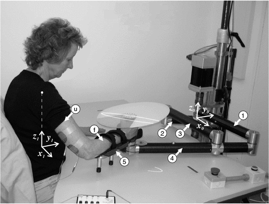
Fig. 4.1

Unimpaired subject using the robotic workstation

Forces of up to 200 N applied in the horizontal plane can be measured with a resolution of 0.0122 N. The fifth link also contains a 4000-line encoder to measures its angle and Light Emitting Diodes (LEDs) to provide visual feedback of the tracking performance. The robotic arm is used to constrain the patient’s arm, to impose forces on the end-effector that make the task feel ‘natural’ to the patient, to apply assistance during the performance of tracking tasks and to move the patient’s arm when necessary. During a treatment session, the patient’s task is to track a range of trajectories that are projected onto a target positioned above their hand. All tests are controlled using a graphical user interface running on the host PC.

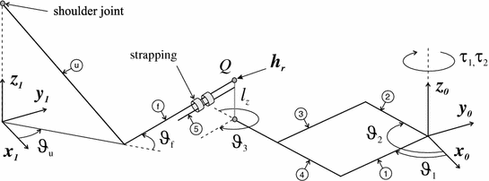
Figure 4.2 shows the geometry of the dual human and robotic system. The robot joint angle vector is $\varvec{q}_r = \left[ \vartheta _1 \; \vartheta _2 \right] ^T$ , where $\vartheta _1$ and $\vartheta _2$ are the joint angles corresponding to links 1 and 2 respectively. Moreover, the axes of all the robot joints are parallel to $\varvec{z}_{0}$ , and the links are labeled to correspond with Fig. 4.1. Also the torque supplied by the motors is given by $\varvec{ \tau }_r = \left[ \tau _1 \; \tau _2 \right] ^T$ , where $\tau _1$ and $\tau _2$ are applied to actuate joints 1 and 2 respectively.

Fig. 4.2

Geometry of combined human arm and robotic arm system

It is assumed that the patient interacts with the robot by applying a vector of forces and torques at the point Q, which has a $\varvec{z}_0$ component of

. This corresponds to the vertical distance of the patient’s hand above the force/torque sensor. The vector of the components of these forces applied in the $\varvec{x}_0$ and $\varvec{y}_0$ directions is given by $\varvec{h}_r$ . The patient’s arm is strapped to the fifth link of the robot and the human arm model therefore includes the properties of this link, which will not be included in the model of the robot. To ensure the robot’s safe interaction with an unknown environment, a form of impedance control, detailed in Colgate and Hogan (1988), is used to govern the torque demand supplied to the motors. This strategy has previously been used to control robotic therapy devices (Krebs et al. 1998), although alternative approaches could be used, such as force or compliant control, e.g., Siciliano and Villani (1999).

The controller compensates for the inertial and damping properties of the robotic arm and at point Q, yields dynamics

$\begin{aligned} \varvec{h}_r = \varvec{K}_{K_x} \tilde{ \varvec{x} }_r + \varvec{K}_{B_x} \dot{ \tilde{ \varvec{x} }}_r + \varvec{K}_{M_x} \ddot{ \tilde{ \varvec{x} }}_r \end{aligned}$

(4.1)

where $\hat{\varvec{x}}_r$ is the reference position, $\tilde{ \varvec{x} }_r = \hat{\varvec{x}}_r - \varvec{x}_r$ , $\varvec{x}_r = \varvec{k}_r ( \varvec{q}_r )$ , $\dot{ \varvec{x} }_r = \varvec{J}_r(\varvec{q}_r) \dot{\varvec{q}}_r$ and $\ddot{ \varvec{x} }_r = \varvec{J}_r(\varvec{q}_r) \ddot{\varvec{q}}_r + \dot{\varvec{J}}_r( \varvec{q}_r,\dot{\varvec{q}}_r) \dot{\varvec{q}}_r$ . Also the direct kinematics equation for the robotic system is $\varvec{x}_r = \varvec{k}_r(\varvec{q}_r)$ and $\varvec{J}_r^T (\varvec{q}_r)$ is the Jacobian of this system. When the robot is moved freely by the patient in the absence of assistance, the gain matrices are set as $\varvec{K}_{K_x} = \varvec{0}$ , $\varvec{K}_{B_x} = K_{B_x} \varvec{I}$ and $\varvec{K}_{M_x} = K_{M_x} \varvec{I}$ , where $\varvec{I}$ is the identity matrix of compatible dimensions. The values of $$$K_{B_x} > 0$$” src=”/wp-content/uploads/2016/09/A306304_1_En_4_Chapter_IEq30.gif”></SPAN> and <SPAN id=IEq31 class=InlineEquation><IMG alt=$ 0$$” src=”/wp-content/uploads/2016/09/A306304_1_En_4_Chapter_IEq31.gif”> are tuned to create a ‘natural’ feel, and an additional requirement is that $\hat{\varvec{x}}_r$ has constant value. Moreover, the robot is required to move the patient’s arm along predefined trajectories. Hence it is necessary to set $\varvec{K}_{K_x} = K_{K_x} \varvec{I}$ with $$$K_{K_x} > 0$$” src=”/wp-content/uploads/2016/09/A306304_1_En_4_Chapter_IEq34.gif”></SPAN> and the three gains tuned to produce the required tracking performance. Gain matrix selection for the case where the robot applies assistance during tracking tasks is described below. </DIV><br /> <DIV></DIV><br /> <DIV id=Sec3 class=$

4.2 Human Arm Model

In this section a mathematical description of the patient’s arm is derived, consisting of a model of the passive dynamical system to which the torque generating properties of the stimulated muscle is then added. This section is based on research reported in Freeman et al. (2007, 2009b).

4.2.1 Passive System

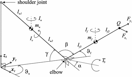
Figure 4.3 gives a more detailed description of the geometry of the constrained human arm model of Fig. 4.2, where the first link represents the upper arm, from the shoulder joint to the elbow, with length $(l_{u1} + l_{u2})$ and the second represents the forearm, from the elbow to the thumb web, with length $(l_{f1} + l_{f2})$ . The constraint means that the forearm must lie in the horizontal plane and rotation is possible about the axis along the upper arm. Point Q denotes where the patient’s hand grasps the robot and only forces and torques along unconstrained directions are shown (only rotation about the axis parallel to $\varvec{z}_{1}$ is unconstrained at this point, rotation is not possible about the two orthogonal axes). The triceps muscle has been selected for stimulation since stroke patients typically experience problems with shoulder and elbow extension during reaching tasks (Lum et al. 2004).

Actuation of the triceps muscle is modeled as a torque, $T_{\beta } \ge 0$ , acting about an axis orthogonal to both the upper arm and forearm. Components of the forces in the $\varvec{x}_{1}$ and $\varvec{y}_{1}$ directions applied by the patient’s hand at the point of interaction with the robot are denoted by $F_{x_{1}}$ and $F_{y_{1}}$ respectively. A point, $\varvec{x}_r$ , in the robot coordinate system is expressed in the human arm system by a point, $\varvec{x}_a$ , such that

$\begin{aligned} \varvec{x}_r = \varvec{x}_a + \left[ \begin{array}{ccc} l_x&l_y&l_{z} \end{array} \right] ^T \end{aligned}$

(4.2)

where

and

represent the $\varvec{x}_{0}$ and $\varvec{y}_{0}$ components, respectively, of the shoulder joint position in the robot coordinate system.

Fig. 4.3

Geometry of constrained human arm

If $\varvec{V}_u$ and $\varvec{V}_f$ are vectors aligned along the upper arm and forearm, respectively, the horizontal constraint requires that $\varvec{V}_f$ has a $\varvec{z}_1$ component of zero. In this case the unitary axis about which $T_{\beta }$ is applied is given by

$\begin{aligned} \varvec{V}_{e} = \frac{ \varvec{V}_u \times \varvec{V}_f }{ | \varvec{V}_u \times \varvec{V}_f |} = \frac{ 1 }{\sqrt{1 - c_f^2 c_{\gamma }^2}} \left[ \begin{array}{ccc} -s_{u f} s_{\gamma }&c_{u f} s_{\gamma }&-s_f c_{\gamma } \end{array} \right] ^T \end{aligned}$

(4.3)

where

and $c_{\gamma }$ denote $\cos (\vartheta _f)$ and $\cos (\gamma ),$ respectively. Similarly, $$s_f$$

and $s_{\gamma }$ denote $\sin (\vartheta _f)$ and $\sin (\gamma )$ . In addition, $$c_u$$

and

are used to denote $\cos (\vartheta _u)$ and $\sin (\vartheta _u),$ respectively, and $s_{uf}$ and $c_{uf}$ denote $\sin (\vartheta _u + \vartheta _f)$ and $\cos (\vartheta _u + \vartheta _f),$ respectively. For arbitrary $\gamma$ , $\varvec{V}_{e}$ has a $\varvec{z}_1$ component of zero when $\vartheta _f = 0$ and is given by

$\begin{aligned} \hat{\varvec{V}}_{e} = \left[ \begin{array}{ccc} -s_{u}&c_{u}&0 \end{array} \right] ^T \end{aligned}$

(4.4)

As $\vartheta _f$ increases, the angle that $\varvec{V}_{e}$ rotates about the upper arm, starting from $\hat{\varvec{V}}_{e}$ , is given by

$\begin{aligned} \alpha ( \vartheta _f ) = \arccos \left( \frac{ \varvec{V}_e \cdot \hat{\varvec{V}}_{e} }{ | \varvec{V}_e | | \hat{\varvec{V}}_{e} |} \right) = \arccos \left( \frac{c_f s_{\gamma }}{\sqrt{1 - c_f^2 c_{\gamma }^2}} \right) \end{aligned}$

(4.5)

The elbow angle is equal to

$\begin{aligned} \beta ( \vartheta _f ) = \arccos \left( \frac{\varvec{V}_u \cdot \varvec{V}_f }{ | \varvec{V}_u | | \varvec{V}_f | } \right) = \arccos \left( - c_f c_{\gamma } \right) \end{aligned}$

(4.6)

and the dynamic model of the constrained arm can be written in the form

(4.7)

where $\varvec{q}_a = [\vartheta _u \; \vartheta _f]^T$ , $\varvec{\tau }_a = \left[ 0 \; T_{\beta } \frac{ - s_f c_{\gamma }}{\sqrt{1 - c_f^2 c_{\gamma }^2}} \right] ^T$ , $\varvec{h}_a = [F_{x_{1}} \; F_{y_{1}}]^T$ and the remaining terms are

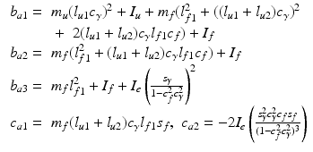
$\begin{aligned} \varvec{B}_a(\varvec{q}_a )&= \left[ \begin{array}{cc} b_{a1} &{}b_{a2} \\ b_{a2} &{}b_{a3} \end{array} \right] ,\,\, \varvec{C_a}(\varvec{q}_a,\dot{\varvec{q}}_a) = \left[ \begin{array}{cc} -2 c_{a1} \dot{\vartheta }_f &{}- c_{a1} \dot{\vartheta }_f \\ c_{a1} \dot{\vartheta }_u &{}c_{a2} \dot{\vartheta }_f \end{array} \right] \end{aligned}$

(4.8)

$\begin{aligned} \varvec{J}_a^T (\varvec{q}_a)&= \left[ \begin{array}{cc} -(l_{u1} + l_{u2}) c_{\gamma } s_u - (l_{f1} + l_{f2}) s_{uf} &{} \;\; (l_{u1} + l_{u2}) c_{\gamma } c_u + (l_{f1} + l_{f2}) c_{uf} \\ -(l_{f1} + l_{f2}) s_{uf} &{}(l_{f1} + l_{f2}) c_{uf} \end{array} \right] \end{aligned}$

(4.9)

with

$\begin{aligned} \begin{array}{rl} b_{a1} = &{}m_u (l_{u1} c_{\gamma })^2 + I_u + m_f (l_{f1}^2 + ((l_{u1} + l_{u2}) c_{\gamma })^2 \\ &{}+\; 2 (l_{u1} + l_{u2}) c_{\gamma } l_{f1} c_f) + I_f \\ b_{a2} = &{}m_f(l_{f1}^2 + (l_{u1} + l_{u2}) c_{\gamma } l_{f1} c_f) + I_f \\ b_{a3} = &{}m_f l_{f1}^2 + I_f + I_e \left( \frac{s_{\gamma }}{1 - c_f^2 c_{\gamma }^2} \right) ^2 \\ c_{a1} = &{}m_f (l_{u1} + l_{u2}) c_{\gamma } l_{f1} s_f,\,\, c_{a2} = -2 I_e \left( \frac{s_{\gamma }^2 c_{\gamma }^2 c_f s_f}{(1 - c_f^2 c_{\gamma }^2)^3} \right) \end{array} \end{aligned}$

(4.10)

The relationship $\varvec{h}_a = - \varvec{h}_r$ is a consequence of the connection between the robotic and human arm systems. Various forms of the friction term $\varvec{F}_{a} ( \varvec{q}_a , \dot{\varvec{q}}_a )$ have been considered to achieve a compromise between repeatability and the accuracy of the overall model. The most general form considered is

$\begin{aligned} \varvec{F}_{a} ( \varvec{q}_a , \dot{\varvec{q}}_a ) = \left[ \begin{array}{cc} F_{a1}(\vartheta _u,\dot{ \vartheta }_u)&F_{a2}(\vartheta _f,\dot{ \vartheta }_f ) \end{array} \right] ^T \end{aligned}$

(4.11)

where $F_{a1}(\cdot )$ and $F_{a2}(\cdot )$ are piecewise linear functions.

4.2.2 Muscle Model

To account for the action of the triceps, an established model of the torque, $T_{\beta }$ , generated by electrically stimulated muscle acting about a single joint is given by

$\begin{aligned} T_{\beta }(\beta ,\dot{\beta },u,t) = g(u,t) \times F_{ma}( \beta ,\dot{\beta } ) + F_{mp}( \beta ,\dot{\beta } ) \end{aligned}$

(4.12)

where u denotes the stimulation pulsewidth applied and $\beta$ is the joint angle (Shue et al. 1995). In this model a Hammerstein structure incorporating a static non-linearity, $h_{\textit{IRC}}(u)$ , representing the isometric recruitment curve, cascaded with linear activation dynamics, $h_{\textit{LAD}}(t)$ , produces the first term, g(u, t). The activation dynamics can be adequately captured using a critically damped second order system as described in, e.g., Baratta and Solomonow (1990), the term $F_{ma} ( \beta ,\dot{\beta } )$ models the multiplicative effect of the joint angle and joint angular velocity on the active torque developed by the muscle and the term $F_{mp} ( \beta , \dot{ \beta } )$ accounts for the passive properties of the joint.

Given that $\gamma$ is invariant, (4.6) means that $F_{mp}( \beta ,\dot{ \beta } )$ is accounted for by the most general form of $\varvec{F}_{a} ( \varvec{q}_a , \dot{\varvec{q}}_a )$ considered. Hence additional forms of friction are not added to the existing model. Details of the procedures used to establish the parameters of the muscle model given above are detailed in Freeman et al. (2007) and further results on the use of system identification to determine a model for the muscle response can be found in Le et al. (2010, 2012).

4.2.3 Robotic Assistance and Trajectory Choice

The action of the robotic arm necessary to make the task a feasible yet productive one is the subject of this section, where the following points concern the choice of trajectory and role of the robot during task completion:

The trajectories will be elliptical reaching tasks for each patient’s dominant arm and should be achievable given their identified arm model.

The triceps muscle will provide the only actuating torque about the elbow and the robotic arm will use the control action given by (4.1) to make the dynamics about the elbow feel ‘natural’ to the patient.

The robotic arm will provide a torque acting about the patient’s shoulder to track the reference in a manner entirely governed by the angle of the forearm, which makes the task feasible without lessening the role played by the triceps.

The development of the robotic control scheme to achieve these goals is described next.

4.2.4 Robotic Control Scheme

Combining the human arm model described by (4.7) and the end effector dynamics (4.1) gives

$\begin{aligned} \varvec{B}_a (\varvec{q}_a ) \ddot{\varvec{q}}_a + \varvec{C}_a(\varvec{q}_a,\dot{\varvec{q}}_a) \dot{\varvec{q}}_a + \varvec{F}_{a} (\varvec{q}_a,\dot{\varvec{q}}_a) = \varvec{\tau }_a + \varvec{J}_a^T (\varvec{q}_a) \Big ( \varvec{K}_{K_x} \tilde{\varvec{x}}_a + \varvec{K}_{B_x} \dot{\tilde{\varvec{x}}}_a + \varvec{K}_{M_x} \ddot{\tilde{\varvec{x}}}_a \Big ) \end{aligned}$

(4.13)

where $\hat{\varvec{x}}_a = \hat{\varvec{x}}_r - [l_x \; l_y \; l_{z}]^T$ has been enforced to give $\tilde{\varvec{x}}_a = \tilde{\varvec{x}}_r$ . To separate the dynamics of the end-effector in the directions corresponding to the human arm joint angles, requires

$\begin{aligned} \varvec{K}_{K_x} \tilde{\varvec{x}}_a + \varvec{K}_{B_x} \dot{\tilde{\varvec{x}}}_a + \varvec{K}_{M_x} \ddot{\tilde{\varvec{x}}}_a = \varvec{J}_a^{-T} (\varvec{q}_a) \Big ( \varvec{K}_{K_q} \tilde{\varvec{q}}_a + \varvec{K}_{B_q} \dot{\tilde{\varvec{q}}}_a + \varvec{K}_{M_q} \ddot{\tilde{\varvec{q}}}_a \Big ) \end{aligned}$

(4.14)

where $\tilde{\varvec{q}}_a = \hat{\varvec{q}}_a - \varvec{q}_a$ and $\hat{\varvec{q}}_a = \varvec{k}^{-1}_a(\hat{\varvec{x}}_a)$ . Hence

$\begin{aligned} \varvec{B}_a (\varvec{q}_a ) \ddot{\varvec{q}}_a + \varvec{C}_a(\varvec{q}_a,\dot{\varvec{q}}_a) \dot{\varvec{q}}_a + \varvec{F}_{a} (\varvec{q}_a,\dot{\varvec{q}}_a) = \varvec{\tau }_a + \varvec{K}_{K_q} \tilde{\varvec{q}}_a + \varvec{K}_{B_q} \dot{\tilde{\varvec{q}}}_a + \varvec{K}_{M_q} \ddot{\tilde{\varvec{q}}}_a \end{aligned}$

(4.15)

and to satisfy the requirements of points 2 and 3 above requires

$\begin{aligned} \varvec{K}_{K_q}&= \left[ \begin{array}{cc} K_{K_1} &{} 0\\ 0 &{} 0 \end{array} \right] , \,\,\, \varvec{K}_{B_q} = \left[ \begin{array}{cc} K_{B_1}&K_{B_2} \end{array} \right] \nonumber \\ \varvec{K}_{M_q}&= \left[ \begin{array}{cc} K_{M_1} &{} 0\\ 0 &{} K_{M_2} \end{array} \right] \end{aligned}$

(4.16)

with $\hat{\varvec{q}}_a = \left[ \hat{\vartheta }_u \; c \right] ^T,$ where c is a constant and $K_{K_1}, K_{B_1}, K_{B_2}, K_{M_1}, K_{M_2} \ge 0$ . This allows a choice of arbitrary second order dynamics to be imposed about the shoulder and the damping and inertia about the elbow to be prescribed.

The right-hand side of (4.15) now is

$\varvec{\tau }_a + \left[ \begin{array}{c} K_{K_1} \tilde{\vartheta }_u + K_{B_1} \dot{\tilde{\vartheta }}_u + K_{M_1} \ddot{\tilde{\vartheta }}_u \\ - K_{B_2} \dot{\vartheta }_f - K_{M_2} \ddot{\vartheta }_f \end{array} \right]$

and gives the required dynamic relationship for both components of the torque on the assumption that $\hat{\vartheta }_f = c$ and therefore $\dot{\hat{\vartheta }}_f = \ddot{\hat{\vartheta }}_f = 0$ . This last assumption is unsuitable for the desired references and hence this control scheme is not appropriate for the intended tracking task. Alternatively, assuming that $\dot{\hat{\vartheta }}_u$ and $\ddot{\hat{\vartheta }}_u$ are sufficiently small, the controller can still provide asymptotic stability to externally applied forces if the right-hand side of (4.15) is

$\varvec{\tau }_a + \left[ \begin{array}{c} K_{K_1} \tilde{\vartheta }_u - K_{B_1} \dot{\vartheta }_u - K_{M_1} \ddot{\vartheta }_u \\ - K_{B_2} \dot{\vartheta }_f - K_{M_2} \ddot{\vartheta }_f \end{array} \right]$

This last requirement is satisfied if $\hat{\varvec{q}}_a = \left[ \hat{\vartheta }_u \; \hat{\vartheta }_f \right] ^T$ and (4.1) is replaced by

$\begin{aligned} \varvec{h}_r = \varvec{K}_{K_x} \tilde{ \varvec{x} }_r - \varvec{K}_{B_x} \dot{ \varvec{x} }_r - \varvec{K}_{M_x} \ddot{ \varvec{x} }_r \end{aligned}$

(4.17)

In this case (4.14) is replaced by

$\begin{aligned} \varvec{K}_{K_x} \tilde{\varvec{x}}_a - \varvec{K}_{B_x} \dot{\varvec{x}}_a - \varvec{K}_{M_x} \ddot{\varvec{x}}_a = \varvec{J}_a^{-T} (\varvec{q}_a) \Big ( \varvec{K}_{K_q} \tilde{\varvec{q}}_a - \varvec{K}_{B_q} \dot{\varvec{q}}_a - \varvec{K}_{M_q} \ddot{\varvec{q}}_a \Big ) \end{aligned}$

(4.18)

and the required values of $\hat{\vartheta }_u$ and $\hat{\vartheta }_f$ are obtained by comparing the components of (4.18) as

$\begin{aligned} \varvec{K}_{K_x} \left( \hat{\varvec{x}}_a - \varvec{x}_a \right) = \varvec{J}_a^{-T} (\varvec{q}_a) \left[ \begin{array}{c} K_{K_1} \left( \hat{\vartheta }_u - \vartheta _u \right) \\ 0 \end{array} \right] = \frac{K_{K_1} \left( \hat{\vartheta }_u - \vartheta _u \right) }{ (l_{u1}+l_{u2})c_{\gamma } s_f } \left[ \begin{array}{c} c_{uf} \\ s_{uf} \end{array} \right] . \end{aligned}$

(4.19)

Hence

$\begin{aligned} \varvec{K}_{K_x} = \frac{K_{K_1} \left( \hat{\vartheta }_u - \vartheta _u \right) }{ \left| \hat{\varvec{x}}_a - \varvec{x}_a \right| (l_{u1}+l_{u2})c_{\gamma } s_f } \varvec{I} \end{aligned}$

(4.20)

and

$\begin{aligned} \hat{\varvec{x}}_a = \varvec{x}_a + \left| \hat{\varvec{x}}_a - \varvec{x}_a \right| \left[ \begin{array}{c} c_{uf} \\ s_{uf} \end{array} \right] \end{aligned}$

(4.21)

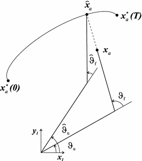
The above analysis shows that $\hat{\varvec{x}}_a$ is not uniquely defined but can be any point lying on a line extending along the forearm and passing through $\varvec{x}_a$ and to meet the tracking task it must be equal to the point of intersection with the trajectory. This requirement is illustrated in Fig. 4.4, where $\varvec{x}_a^*( t ) = \varvec{k}_a (\varvec{q}_a^* (t) )$ and the trajectory is defined by

$\begin{aligned} \varvec{q}_a^* (t) = \left[ \vartheta _u^* (t) \; \vartheta _f^* (t) \right] ^T,\,\, 0 \le t \le T \end{aligned}$

(4.22)

Eliminating t from the components gives $\vartheta _u = \varPsi ( \vartheta _f )$ and the reference is defined formally as

$\begin{aligned} \begin{array}{c} \hat{\varvec{x}}_a = \varvec{\varOmega } \left( \varvec{x}_a , \varPsi ( \cdot ) \right) := \varvec{k}_a \left( \left[ \begin{array}{c} \varPsi ( \hat{\vartheta }_f ) \\ \hat{\vartheta }_f \end{array} \right] \right) \\ \bigg | \varvec{k}_a \left( \left[ \begin{array}{c} \varPsi ( \hat{\vartheta }_f ) \\ \hat{\vartheta }_f \end{array} \right] \right) = \varvec{x}_a + \lambda \left[ \begin{array}{c} c_{uf} \\ s_{uf} \end{array} \right] \end{array} \end{aligned}$

(4.23)

where $\lambda$ is a scalar.

Fig. 4.4

Trajectory geometry

The final control system is shown in Fig. 4.5 where, given (4.16),

$\begin{aligned} \varvec{K}_{B_x} = \varvec{J}_a^{-T} (\varvec{q}_a) \varvec{K}_{B_q} \varvec{J}_a^{-1} (\varvec{q}_a) \end{aligned}$

(4.24)

and

$\begin{aligned} \varvec{K}_{M_x} \left( \varvec{J}_a (\varvec{q}_a) \ddot{\varvec{q}}_a + \dot{\varvec{J}}_a (\varvec{q}_a,\dot{\varvec{q}}_a) \dot{\varvec{q}}_a \right) = \varvec{J}_a^{-T} (\varvec{q}_a) \varvec{K}_{M_q} \end{aligned}$

(4.25)

Also, using (4.23), (4.20) can be written explicitly as

$\begin{aligned} \varvec{K}_{K_x} \left( \varvec{x}_a , \varPsi ( \cdot ) \right) = \frac{K_{K_1} \left( \varPsi ( \hat{\vartheta }_f) - \vartheta _u \right) }{ \lambda (l_{u1}+l_{u2})c_{\gamma } s_f } \varvec{I} \end{aligned}$

(4.26)

Fig. 4.5

Human arm system with robotic assistance

Fig. 4.6

Approximate model of the stimulated human arm

4.2.5 Trajectory Selection for ILC Design

How the trajectories feel to the patient is critical and impacts on the selection of $K_{B_2}$ and $K_{M_2}$ as follows:

For $\varPsi ( \vartheta _f )$ to be a one-one continuous function, both $\vartheta _u^* (t)$ and $\vartheta _f^* (t)$ must be monotone.

With the use of robotic assistance, it is shown in Freeman et al. (2009c) that the behavior of the electrically stimulated tricep can be approximated by the system represented schematically in Fig. 4.6. The approximations invoked are based on experimentally confirmed properties of the human arm model and the ability of the robotic control system to provide accurate tracking of $\hat{\vartheta }_u$ by $\vartheta _u$ .

Given $T_{\beta } \ge 0$ , 1) above requires that $\vartheta _f^* (t)$ is monotonically decreasing. Moreover, given the geometry of the task shown in Fig. 4.4, this last requirement requires that the line joining $\varvec{x}_a^*(T)$ and $\varvec{x}_a^*(0)$ passes through the origin of the arm system, since at both these points the direction of the elliptical trajectory is orthogonal to the major axis.

Under the assumption that $\vartheta _f^* (t)$ is tracked perfectly, the torque that must be applied to the arm system shown in Fig. 4.6 is given by

$\begin{aligned} T_{\beta }^*(t) \approx \left( \frac{ - \sqrt{1 - c^2_{f^*(t)} c^2_{\gamma }}}{s_{f^*(t)} c_{\gamma }} \right)&\Big \{ K_{B_2} \dot{ \vartheta }_f^*(t) + \big ( K_{M_2} + b_{a3} \big ) \ddot{ \vartheta }_f^*(t)\nonumber \\&\quad + F_{a2} \left( \vartheta _f^*(t),\dot{\vartheta }_f^*(t) \right) \Big \} \ \end{aligned}$

(4.27)

and the required stimulation, $$u^*(t)$$

, must satisfy

$\begin{aligned} \int _0^t h_{IRC} \left( u^*( \tau ) \right) h_{LAD} \left( t - \tau \right) d \tau = \frac{ T_{\beta }^* (t) }{ F_{ma}(\beta ^* (t) ,\dot{ \beta }^* (t)) } \end{aligned}$

(4.28)

where $\beta ^*(t)$ corresponds to the reference trajectory such that $\beta ^*(t)\! = \beta ( \vartheta _f^* (t),t)$ . This expression limits the magnitude and rate of change of any achievable torque trajectory.

In application the existence of a solution to (4.28) will be ensured by selecting slow trajectories that comprise half ellipse segments that are comfortably within both the robot’s and the patient’s workspace. The start and end points will be chosen such that they can be reached by a smooth extension of the elbow and individually calculated for each patient depending on their maximum reach capability. Moreover, the gains $K_{B_2}$ and $K_{M_2}$ are selected to: (i) mimic a realistic activity, (ii) provide a high level of stability in response to sudden stimulation inputs and (iii) to require that a moderate level of work is generated by the patient’s muscles in order to track the trajectory.

The effects of these requirements on the overall control scheme will discussed later in the chapter.

4.3 Control Laws

In this section, two strategies to control the stimulation applied to the patient are developed. The first consists of a linearizing controller in a simple structure feedback arrangement and the second augments this arrangement by adding an ILC feedforward action generated by one of two laws.

4.3.1 Linearizing Control Law

The first component of this control law is $h_{\textit{IRC}}^{-1} ( \cdot )$ , which is the inverse of the isometric recruitment curve that has been identified for each patient and the remaining action of the control law is motivated by the form of the remaining non-linear terms $-s_{f} c_{\gamma } / \sqrt{1 - c^2_{f} c^2_{\gamma }}$ , $F_{ma}(\beta , \dot{\beta })$ and $F_{a2} (\vartheta _{f},\dot{\vartheta }_{f})$ of the arm model of Fig. 4.6. The value of all three functions vary only slowly when the trajectories considered in this chapter are followed perfectly (Freeman et al. 2007), where this conclusion is based on examining the graphs of each function using the substitutions $\vartheta _f = \vartheta _f^*(t)$ , $\dot{\vartheta }_f = \dot{\vartheta }_f^*(t)$ , $\beta = \beta ^*(t)$ and $\dot{\beta } = \dot{\beta }^*(t)$ for the trajectories used.

The control action taken attempts to remove the effect of these functions and hence produce a system that approximates the linear activation dynamics in series with the linear arm dynamics (the transfer-functions appearing in the left and right sub-systems, respectively, of Fig. 4.6). To achieve this, the control law next applies the gain term

$\begin{aligned} \frac{ - \sqrt{1 - c^2_{{f}} c^2_{\gamma }}}{s_{{f}} c_{\gamma } F_{ma}({\beta } ,\dot{{\beta }})} = \left( -s_{f} c_{\gamma } / \sqrt{1 - c^2_{f} c^2_{\gamma }} \right) ^{-1} \left( F_{ma}(\beta , \dot{\beta }) \right) ^{-1} \end{aligned}$