Fig. 3.1
Feedback control scheme with 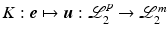
This chapter addresses the design of feedback controllers to stabilize all joints in the upper limb system. Moreover, robust stability margins are derived to ensure that changes in the dynamics do not destabilize the system. To maximize practical utility, these are employed to derive bounds on the most significant sources of model inaccuracy, with explicit focus on muscle fatigue. In the next chapter a feedforward control action will be combined with the feedback controllers developed here in order to further improve tracking accuracy and hence ensure successful task completion.
3.1 General Feedback Control Framework
The combined mechanical and anthropomorphic system was shown to take the form
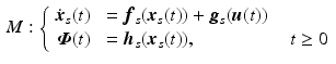
with components given by (2.7). Since  are continuously differentiable, M has the properties of uniqueness and continuity [11]. In this chapter we consider a general feedback control structure given by
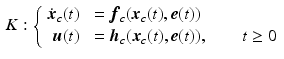
where functions  are continuously differentiable, so that K also has the properties of uniqueness and continuity. Figure 3.1 shows the combined structure, where the reference vector is denoted
  and the tracking error is
  . This must be designed to embed robustness to model uncertainty and disturbance, together with baseline tracking performance of the resulting closed-loop system
![$$\begin{aligned} \underbrace{ \left[ \begin{array}{c} \dot{\varvec{x}}_{s}(t) \\ \dot{\varvec{x}}_{c}(t) \end{array} \right] }_{\displaystyle { \dot{\varvec{x}}(t) }}&= \underbrace{ \left[ \begin{array}{c} \varvec{f}_s ( \varvec{x}_{s}(t) ) + \varvec{g}_s ( \varvec{h}_c ( \varvec{x}_{c}(t), \hat{\varvec{\varPhi }}(t) - \varvec{h}_s ( \varvec{x}_{s}(t) ) ) ) \\ \varvec{f}_c ( \varvec{x}_{c}(t), \hat{\varvec{\varPhi }}(t) - \varvec{h}_s ( \varvec{x}_{s}(t) ) ) \end{array} \right] }_{\displaystyle { \varvec{f} ( \varvec{x}(t), \hat{\varvec{\varPhi }}(t) )}} \nonumber \\ \varvec{\varPhi }(t)&= \underbrace{ \varvec{h}_s ( \varvec{x}_{s}(t) ) }_{\displaystyle { \varvec{h} ( \varvec{x}(t) ) }}, \quad \quad t \ge 0. \end{aligned}$$](/wp-content/uploads/2016/09/A352940_1_En_3_Chapter_Equ3.gif)
The functional movements used in rehabilitation may not involve all joint axes. Equally movement about certain joints may need to be actively avoided, due to the presence of subluxations, stiffness, or limited angular range of movement for example. To embed this flexibility in controlled joint selection, we define the set  containing the controlled joint indices, with elements
  ,
,  . We denote the complement of
  by
by  . For signal
  and set of distinct indices
  we use notation
 ![$$\varvec{x}_\mathscr {S}(t) = [\varvec{x}_{\mathscr {S}(1)}(t), \ldots \varvec{x}_{\mathscr {S}_{|\mathscr {S}|}}(t)]^\top $$](/wp-content/uploads/2016/09/A352940_1_En_3_Chapter_IEq13.gif) where
where  is the ith smallest element of
  . With this notation, the controlled and uncontrolled joint angle signals are
  and
and  respectively. Armed with this notation, we can now introduce a definition of stability for use in control design:
(3.1)
are continuously differentiable, M has the properties of uniqueness and continuity [11]. In this chapter we consider a general feedback control structure given by(3.2)
are continuously differentiable, so that K also has the properties of uniqueness and continuity. Figure 3.1 shows the combined structure, where the reference vector is denoted and the tracking error is . This must be designed to embed robustness to model uncertainty and disturbance, together with baseline tracking performance of the resulting closed-loop system(3.3)
containing the controlled joint indices, with elements , . We denote the complement of by . For signal and set of distinct indices we use notation where is the ith smallest element of . With this notation, the controlled and uncontrolled joint angle signals are and respectively. Armed with this notation, we can now introduce a definition of stability for use in control design:Definition 3.1
Feedback controller (3.2) is said to stabilize the closed-loop system [M, K] about operating-point  if it achieves global asymptotic stability of the controlled joints,
  , about
  .
.
if it achieves global asymptotic stability of the controlled joints, , about .Satisfying the condition of Definition 3.1 stabilizes joints with indices in set  , but musculo-tendon interaction and dynamic rigid body coupling cause movement in the remaining joints. We therefore next derive conditions to ensure stability of the uncontrolled joints,
  ,
,  .
.
, but musculo-tendon interaction and dynamic rigid body coupling cause movement in the remaining joints. We therefore next derive conditions to ensure stability of the uncontrolled joints, , .3.1.1 Stability of Unactuated Joints
To examine stability of uncontrolled joints,  ,
,  , first express components of
  in standard form as
where  are components of
  . Then using
  ,
, ![$$\varvec{\eta } = [\varvec{\eta }_1^\top , \; \varvec{\eta }_2^\top ]^\top $$](/wp-content/uploads/2016/09/A352940_1_En_3_Chapter_IEq30.gif) ,
, ![$$\varvec{\xi } = [ \varvec{\xi }_1^\top , \; \varvec{\xi }_2^\top , \; \varvec{\xi }_3^\top ]^\top $$](/wp-content/uploads/2016/09/A352940_1_En_3_Chapter_IEq31.gif) , the system (2.7) and controller (3.2) can be represented as
, the system (2.7) and controller (3.2) can be represented as

![$$\begin{aligned} \varvec{\xi } (\varvec{x})= & {} \left[ \begin{array}{c} \bar{\varvec{\varPhi }} - \varvec{\varPhi }_{ \mathscr {P}} \\ \bar{\varvec{\varPhi }}^{(1)} - \varvec{\varPhi }_{ \mathscr {P}}^{(1)} \\ \bar{\varvec{\varPhi }}^{(2)} - \varvec{\varPhi }_{ \mathscr {P}}^{(2)} \end{array} \right] = \left[ \begin{array}{c} \bar{\varvec{\varPhi }} - \varvec{h}_{ \mathscr {P}} (\varvec{x}(t)) \\ \bar{\varvec{\varPhi }}^{(1)} - \varvec{h}_{ \mathscr {P}} ( \varvec{f} ( \varvec{x}(t) )) \\ \bar{\varvec{\varPhi }}^{(2)} - \varvec{h}_{ \mathscr {P}} ( \varvec{f}^\prime ( \varvec{x}(t) ) \varvec{f} ( \varvec{x}(t) )) \end{array} \right] , \end{aligned}$$](/wp-content/uploads/2016/09/A352940_1_En_3_Chapter_Equ7.gif)
where ![$$\varvec{\varPhi } = [ \varvec{\eta }_1^\top , \bar{\varvec{\varPhi }}^\top - \varvec{\xi }_1^\top ]^\top $$](/wp-content/uploads/2016/09/A352940_1_En_3_Chapter_IEq32.gif) ,
, ![$$\dot{\varvec{\varPhi }} = [ \varvec{\eta }_2^\top , (\bar{\varvec{\varPhi }}^{(1)})^\top - \varvec{\xi }_2^\top ]^\top $$](/wp-content/uploads/2016/09/A352940_1_En_3_Chapter_IEq33.gif) , and the uncontrolled joint dynamics are
, and the uncontrolled joint dynamics are
 Terms
Terms  and
and  respectively have elements
 and likewise
  and
and  have elements
Assuming the passive parameter form (2.12),  has elements
 From (3.5)–(3.7) the surface
  defines an integral manifold for the system

Since the controlled joints are assumed to be stable about this surface via Definition 3.1, system (3.9) is globally attractive and defines the zero dynamics relative to the controlled output  . We next state the Center Manifold Theorem, see [12].
, , first express components of in standard form as(3.4)
are components of . Then using , , , the system (2.7) and controller (3.2) can be represented as(3.5)
(3.6)
(3.7)
, , and the uncontrolled joint dynamics are and respectively have elements and have elements(3.8)
has elements defines an integral manifold for the system(3.9)
. We next state the Center Manifold Theorem, see [12].Theorem 3.1


Stability of all joints,  , is hence assured if both the controlled and uncontrolled joints are independently stable. The former is guaranteed via Definition 3.1, and the following theorem gives conditions for the latter.
, is hence assured if both the controlled and uncontrolled joints are independently stable. The former is guaranteed via Definition 3.1, and the following theorem gives conditions for the latter.Theorem 3.2
Let feedback controller K satisfy Definition 3.1 and uncontrolled joints,  , be passive with respect to
  , i.e.

where  satisfies
  , with
  the moment transferred from controlled to uncontrolled joints, and let the uncontrolled joint damping function satisfy the sector bounds
Then the uncontrolled joints are locally stable about  .
.
, be passive with respect to , i.e.(3.10)
satisfies , with the moment transferred from controlled to uncontrolled joints, and let the uncontrolled joint damping function satisfy the sector bounds(3.11)
.Proof
From (2.7) the uncontrolled system dynamics are given by
The term  can be partitioned as
 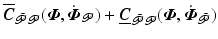 , where
 Furthermore
  can be written as
  with
with
 This enables (3.12) to be rewritten using substitutions
  and
and  , where
  , to give
When  the zero dynamics correspond to the system
where the muscle dynamic forms (2.2)–(2.4) mean  is bounded input, bounded output stable, and functional dependence on
  ,
,  has been omitted. System (3.14) equates to
  where
where
 The equilibrium point of the uncontrolled joints satisfies
  , and, following [13], the system can be interpreted as conservative system
  acted on by external force
  where
where  . Accordingly, introduce energy function
 The first and second terms respectively correspond to the kinetic and potential energy in the uncontrolled joint system, and the third to the potential energy transferred from the controlled joints. The rate of energy satisfies
 Hence the system converges to
  ,
,  if
if
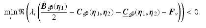 As
As 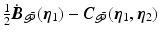 is skew-symmetric, a sufficient condition is that the term
 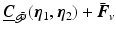 is diagonally dominant with positive diagonal entries, which is satisfied by (3.11).
(3.12)
can be partitioned as , where can be written as with and , where , to give(3.13)
the zero dynamics correspond to the system(3.14)
is bounded input, bounded output stable, and functional dependence on , has been omitted. System (3.14) equates to where, and, following [13], the system can be interpreted as conservative system acted on by external force where . Accordingly, introduce energy function, if is skew-symmetric, a sufficient condition is that the term is diagonally dominant with positive diagonal entries, which is satisfied by (3.11). The conditions of Theorem 3.2 motivate the following intuitive guidelines for ensuring stability of the uncontrolled joints:
Procedure 1
(Design guidelines for stabilizing uncontrolled joints)
Add damping: The condition on  , given by (3.11), can always be met by adding viscous damping to the uncontrolled joints.
, given by (3.11), can always be met by adding viscous damping to the uncontrolled joints.Feedback controller tuning: Bounds on  scale with
  , and hence (3.10) and (3.11) are easy to satisfy if the controlled joint equilibrium trajectory is smooth. This motivates (de)-tuning of feedback controller (3.2).
scale with , and hence (3.10) and (3.11) are easy to satisfy if the controlled joint equilibrium trajectory is smooth. This motivates (de)-tuning of feedback controller (3.2).Reference selection: The controlled joint equilibrium trajectory can also be made smoother through selection of the reference trajectory  .
.
.Arm structure selection: The amount of damping required for stability is dictated by the degree of axis coupling which is reflected in the magnitude of elements  . The components of
  are related to the elements of
  via (3.4). Note that they do not involve components on the principal diagonal of
  and hence the bound is solely dependent on the amount of interaction between the system joints. With no interaction
  , reducing to the requirement that
  is passive.
. The components of are related to the elements of via (3.4). Note that they do not involve components on the principal diagonal of and hence the bound is solely dependent on the amount of interaction between the system joints. With no interaction , reducing to the requirement that is passive.Stimulated muscle selection: Musculo-tendon coupling produces moments  about uncontrolled joints due to applied ES. This solely has the effect of displacing the equilibrium point
  .
.
about uncontrolled joints due to applied ES. This solely has the effect of displacing the equilibrium point .Mechanical support: This also displaces the equilibrium point  , but can also be used to satisfy passivity condition (3.10). Note that the mechanical support must provide sufficient support such that an equilibrium point,
  , exists for the uncontrolled joints.
, but can also be used to satisfy passivity condition (3.10). Note that the mechanical support must provide sufficient support such that an equilibrium point, , exists for the uncontrolled joints.3.2 Case Study: Input-Output Linearizing Controller
The feedback control design approach is next illustrated by applying it to the clinically relevant system that was introduced in Sect. 2.2.5. Here ES is applied to the anterior deltoid and triceps muscles using inputs  and
and  respectively. The kinematics are shown in Fig. 2.3, and the clinical objective is to ensure
  and
and  track reference signals
  and
and  respectively, with the remaining joint angles stable [14, 15]. Hence we set
  ,
,  ,
,  and
and  .
.
and respectively. The kinematics are shown in Fig. 2.3, and the clinical objective is to ensure and track reference signals and respectively, with the remaining joint angles stable [14, 15]. Hence we set , , and .The linear actuation dynamics  ,
,  appearing in dynamic model (2.7) can be assumed to be second order [16], so that without loss of generality
  . This gives rise to the Hammerstein structures
![$$\begin{aligned} \dot{\varvec{x}}_{i}(t)&= \underbrace{\left[ \begin{array}{cc} -d_{i,1} &{} -d_{i,2} \\ 1 &{} 0 \end{array} \right] }_{\varvec{M}_{A,i}} \varvec{x}_{i}(t) + \underbrace{\left[ \begin{array}{c} 1 \\ 0 \end{array} \right] }_{\varvec{M}_{B,i}} h_{{\textit{IRC}},i} ( u_{i}(t) ), \nonumber \\ h_i(u_i,t)&= \underbrace{[ \begin{array}{cc} n_{i,1}&n_{i,2} \end{array} ]}_{\varvec{M}_{C,i}} \varvec{x}_{i}(t), \quad \qquad \qquad \quad \quad \; i \in \{ 1, 2 \}. \end{aligned}$$](/wp-content/uploads/2016/09/A352940_1_En_3_Chapter_Equ15.gif)
We employ musclo-tendon mapping (2.4) and since muscles are aligned with joints
 Using
Using ![$$\varvec{x}_s = [\varvec{\varPhi }^\top , \dot{\varvec{\varPhi }}^\top , \varvec{x}_2^\top , \varvec{x}_5^\top ]^\top $$](/wp-content/uploads/2016/09/A352940_1_En_3_Chapter_IEq102.gif) the controlled dynamics, M, of system (3.1) are hence
the controlled dynamics, M, of system (3.1) are hence
![$$\begin{aligned} \dot{\varvec{x}}_s&= \underbrace{ \left[ \begin{array}{c} \dot{\varvec{ \varPhi }} \\ \varvec{B} ( \varvec{ \varPhi })^{-1} \left( \left[ \begin{array}{c} 0 \\ F_{M,2,1}( \phi _2, \dot{\phi }_2 ) \varvec{M}_{C,1} \varvec{x}_1 \\ 0 \\ 0 \\ F_{M,5,2}( \phi _5, \dot{\phi }_5 ) \varvec{M}_{C,2} \varvec{x}_2 \end{array} \right] - \varvec{X}(\varvec{\varPhi },\dot{\varvec{\varPhi }}) \right) \\ \varvec{M}_{A,1} \varvec{x}_1 \\ \varvec{M}_{A,2} \varvec{x}_2 \end{array} \right] }_{\varvec{f}_s(\varvec{x}_s)} + \underbrace{ \overbrace{ \left[ \begin{array}{cc} 0 &{}0 \\ 0 &{}0 \\ 0 &{}0 \\ 0 &{}0 \\ 0 &{}0 \\ \varvec{M}_{B,1} &{}0 \\ 0 &{}\varvec{M}_{B,2} \end{array} \right] }^{\displaystyle {[g_1(\varvec{x}_s), \; g_2(\varvec{x}_s)]}} \left[ \begin{array}{c} h_{\textit{IRC},1}(u_1) \\ h_{\textit{IRC},2}(u_2) \end{array} \right] }_{\varvec{g}_s(\varvec{u})} \nonumber \\ \varvec{\varPhi }_{ \mathscr {P}}&= \left[ \begin{array}{c} \phi _2 \\ \phi _5 \end{array} \right] = \left[ \begin{array}{c} h_1(\varvec{x}_s) \\ h_2(\varvec{x}_s) \end{array} \right] \end{aligned}$$](/wp-content/uploads/2016/09/A352940_1_En_3_Chapter_Equ16.gif)
where
 To satisfy Definition 3.1, we next design K using input-output linearization in order to control
  using
using ![$$\varvec{u} = [u_1, u_2]^\top $$](/wp-content/uploads/2016/09/A352940_1_En_3_Chapter_IEq104.gif) . As described in [12], for an
. As described in [12], for an  system the control action is
, appearing in dynamic model (2.7) can be assumed to be second order [16], so that without loss of generality . This gives rise to the Hammerstein structures(3.15)
the controlled dynamics, M, of system (3.1) are hence(3.16)
using . As described in [12], for an system the control action is![$$\begin{aligned} \Big [ \begin{array}{c} h_{\textit{IRC},1}(u_1) \\ h_{\textit{IRC},2}(u_2) \end{array} \Big ] = \varvec{\chi }(\varvec{x}_s)^{-1} \big ( \varvec{v} - \varvec{\mu }(\varvec{x}_s) \big ) \end{aligned}$$](/wp-content/uploads/2016/09/A352940_1_En_3_Chapter_Equ17.gif)


