Clinical Wear Assessment

John M. Martell

Introduction

Wear has been a major consideration in total hip arthroplasty since its introduction by Sir John Charnley in the late 1950s. Charnley’s original prosthetic design attempted to limit wear by utilizing a 22.225-mm femoral bearing coupled with the low-friction material Teflon. Unfortunately, Teflon did not have adequate wear resistance and the debris generated elicited an intense inflammatory reaction in the periprosthetic tissues. Sir John Charnley’s subsequent designs used more durable ultrahigh–molecular-weight polyethylene as a bearing counterface (1). Although less reactive to the tissues than Teflon debris, ultrahigh–molecular-weight polyethylene debris elicits an inflammatory response resulting in periprosthetic osteolysis and subsequent prosthetic loosening (1,2,3). In today’s contemporary designs using a highly cross-linked polyethylene insert, clinical wear rates have been reduced by 50% to 90% compared to standard polyethylene (4,5,6,7). At 5 to 10 years of clinical follow-up the incidence of osteolysis in a large series of hips is essentially zero (7,8). Historically, particle-mediated osteolysis and loosening were a primary factor limiting the long-term survival of implants (2,9).

Modifications to the design of the original Charnley low-friction arthroplasty have been shown to influence the polyethylene wear rates. These changes include the material chosen for the articular surface (cobalt chrome, titanium, ceramic) (3), the size of the bearing (22.225 mm, 26 mm, 28 mm, 32 mm) (10), the thickness of the polyethylene (11,12,13), and the propensity for debris generation (bead shedding and third-body wear from nonarticular surfaces and fretting of modular junctions) (14,15). Many of these design changes had an adverse effect on wear performance of the implants. Although catastrophic failure is easily detected on radiographs, it is more difficult to appreciate the short-term effects that design changes have on the polyethylene wear rate in vivo. Although materials testing is a valuable tool for predicting the wear performance of new implant designs, tools for the clinical assessment of wear in patients are also critical. Hip simulators represent our best attempt at re-creating the mechanical environment of a total hip in vivo, yet only recently have simulator wear rate predictions been validated with clinically observed wear rates (4).

Early attempts to correlate clinical and radiographic outcomes with polyethylene wear rates yielded variable results (16,17). Studies with long-term data (>8 to 10 years), demonstrated significant correlations between clinical variables and measured wear rates (10,18,19). Although useful for the assessment of long-term data, manual techniques of polyethylene wear measurement lack the precision and accuracy to assess the impact of design changes on wear performance using short-term data (20). Traditional manual techniques of measuring wear, including the methods of Charnley, Dorr, and Livermore are accurate in experienced hands, but lack the precision necessary to assess wear rates in the short term. It is important to understand the precision and accuracy of measurement techniques used to assess wear, particularly in the era of cross-linked polyethylene with predicted wear rates <60 μm per year.

Assessment of Wear Measurement Techniques

The performance of a measurement instrument can be assessed in terms of precision and bias. Precision is the closeness of agreement between measurements taken under similar conditions whereas bias is the consistent or systematic difference between a set of measurements and an accepted reference value (21). Both precision and bias are fundamental determinants of an instrument’s accuracy. The relationship between precision, bias, and accuracy is demonstrated in Figure 18.1 and Table 18.1.

Bias

Bias is the consistent or systematic difference between a set of measurements and an accepted reference value.

Precision

Precision is defined as the closeness of agreement between repeated independent test results obtained under stipulated conditions. The ASTM standard practice E177-90a recommends precision be expressed using a 95% level of confidence as shown in Equation 1 (21).

where t = t statistic for 95% confidence interval

S_dif = Standard deviation (measured value − true value)

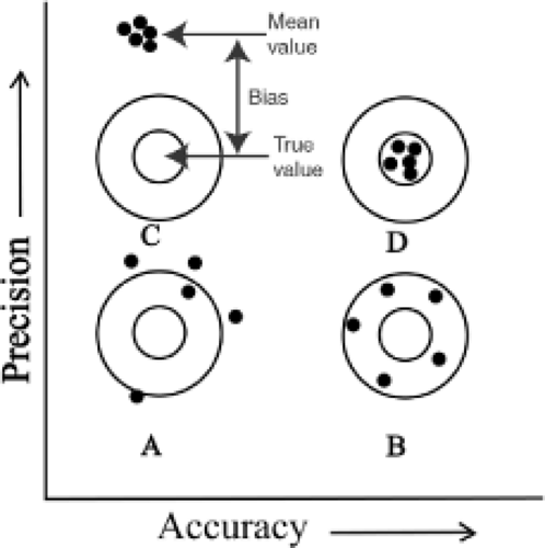Figure 18.1. Instrument A has low accuracy and low precision, whereas B has high accuracy (mean value = true value) but low precision. C demonstrates high precision with poor accuracy, and D is both accurate and precise. Instrument A is unusable whereas instrument B can yield useful data if sample size is adequate and follow-up is sufficient. Instrument C is precise but inaccurate and contains systematic error (bias). If the bias of the instrument can be corrected through calibration, the instrument may yield acceptable data.

Bland and Altman advocate using the 95% confidence interval of the standard error to estimate precision (Equation 2) (22).

where t = t statistic for 95% confidence interval

S_dif = Standard deviation (measured value − true value)

n = Total number of observations

Table 18.1 Sample Data for the Validation of a Wear-Detection Technique^a

Actual Wear (μm)	Measured Wear (μm)	Difference (μm)
0	41	−41
0	19	−19
0	−24	−24
0	−72	−72
50	−47	3
100	−119	−19
150	−107	43
200	−175	25
200	−200	0
200	−225	−25
200	−219	−19
200	−245	−45
200	−177	23
200	−233	−33
200	−212	−12
200	−161	39
	Mean difference	−3.5
	Standard deviation difference	33.4
	Accuracy ±	65.0
	Precision (ASTM)	16.0
	Precision (B&A)	16.4
	RC	66.8
^a This technique consists of little bias (mean difference from standard = −3.5 μm), reasonable precision, and acceptable accuracy.

Accuracy

A standard method of reporting accuracy has not been established in the literature. The ASTM standard recommends reporting bias and precision rather than accuracy. Published wear studies report on the accuracy of their polyethylene wear measurements in a variety of ways, making direct comparisons of accuracy between published techniques difficult. However, when the raw measurement data is given, the standard error, also called the root mean square error, may be calculated (Equation 3) (21).

where x = individual measurement

T = true value for measurement

The 95% confidence limits for accuracy are then estimated by multiplying the standard error by the two-tailed t-statistic with n − 1 degrees of freedom (Equation 4).

where t = two-tailed t statistic at the 95% confidence level with n − 1 degrees of freedom.

Repeatability

This may be reported as the precision within and between observers or as the repeatability coefficient (RC) as defined by Bland and Altman. The RC is defined as two times the standard deviation of the difference between two measurements taken under the same conditions (Equation 5). Repeatability can be calculated for the same observer (intraobserver repeatability) or between different observers (interobserver) (22,23).

where S_dif = standard deviation (measured value − true value)

Standard Components of Variance Analysis

This approach uses analysis of variance to determine the percent variation contributed by each component of the measurement system. The percent measurement variation introduced by the measuring instrument, by the individual measuring the wear, and by variations in patient use are calculated (24). Ideally, in a good measurement system, the variation introduced by the instrument and the observer is less than the variation observed in the wear values as a result of patient clinical factors. Although this technique yields detailed information on sources of potential error, a full analysis is time consuming, requires multiple observations per observer, and multiple observers.

Classifications of Wear Measurement Techniques

Published polyethylene wear studies differ with respect to the technique by which the measurements are made, the
method by which they calculate wear, and the manner in which wear is reported.

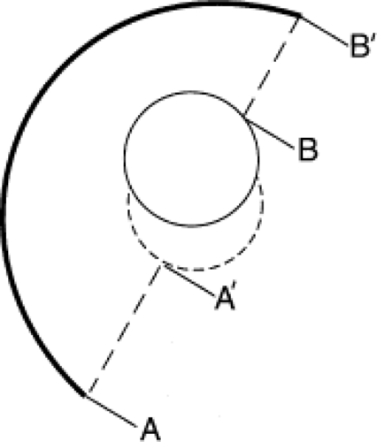Figure 18.2. Wear is calculated by measuring B–B′ and subtracting its value from A–A′. This 2D method requires only one follow-up radiograph, but detects only the component of wear directed toward the margin of the acetabular component (B′).

Weight Bearing

The potential advantage of weight bearing is the assurance that the femoral bearing is in contact with the polyethylene of the acetabular component when the x-ray is acquired. Investigators have reported weight bearing to have both a significant and an insignificant (25,26) effect on wear measurements. Smith et al. showed significantly more wear with standing x-rays than with supine x-rays (27). Digas et al. found a 50% difference between highly cross-linked and conventional polyethylene with standing, but not with supine, radiosteriometric analysis (RSA) studies. In this series the non–weight-bearing films were taken at 1 week postoperatively whereas weight-bearing films were taken from 3 months on, (28) making it difficult to attribute the difference observed entirely to weight bearing. In a prospective direct comparison of standing versus supine AP pelvis films, Moore et al. found no statistically significant difference in the wear measured with standing radiographs (26). Other investigators have shown that load bearing has no reproducible effect on the position of the femoral head in the acetabular component (25). Currently, there is no consensus on the importance of obtaining standing radiographs for wear studies.

Techniques of Analysis

Each measurement method can be classified as either a manual or a computer-assisted technique. Although manual techniques may yield good results in experienced hands, computer-assisted techniques generally provide superior precision and accuracy. Computer-assisted techniques may be classified as those using:

Edge detection
Computer vision
Correction for geometric distortion

Computer-based methods capable of correcting for geometric image distortion will perform well when high-resolution images (300 DPI) are available (29). Radiographic series that lack the resolution necessary for computerized analysis may require analysis by manual techniques.

Method of Analysis

The method for calculating wear can be classified into four types: uniradiographic, which is based on the analysis of one follow-up radiograph (Fig. 18.2), duoradiographic which compares two radiographs to determine the maximum change in polyethylene thickness (Fig. 18.3

Only gold members can continue reading. Log In or Register to continue