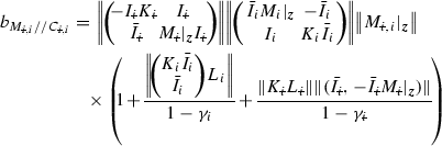
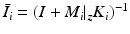
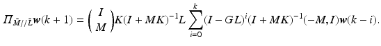
Fig. 9.1
Feedback and ILC control scheme for arbitrary electrode structures
Procedure 9
(Embedding arrays within general robustness framework) Suppose N groups of single-pad electrodes or electrode arrays are used. Let the ith group contain  electrode elements, stimulating
  muscles and have a specified subspace of dimension
  . Then the system can be represented by Fig. 9.1 where operator A is defined by
![$$\begin{aligned}&A : \mathscr {L}^{n}_2[0,T] \rightarrow \mathscr {L}^{m}_2[0,T] : \varvec{z} \mapsto \varvec{u}, \; \varvec{u}_j = A_j \varvec{z}_j, \; j = 1 \ldots N \end{aligned}$$](/wp-content/uploads/2016/09/A352940_1_En_9_Chapter_Equ1.gif)
where  ,
,  , and operator
 ![$$A_j : \mathscr {L}^{n_j}_2[0,T] \rightarrow \mathscr {L}^{m_j}_2[0,T]$$](/wp-content/uploads/2016/09/A352940_1_En_9_Chapter_IEq6.gif) is given by (8.2), where for a group of single-pad electrodes,
is given by (8.2), where for a group of single-pad electrodes,  with
with  for
for  and
and  otherwise. Similarly, operator X is defined as
![$$\begin{aligned}&X : \mathscr {L}^{q}_2[0,T] \rightarrow \mathscr {L}^{n}_2[0,T] : \varvec{r} \mapsto \varvec{z}, \; \varvec{z}_j = X_j \varvec{r}_j, \; j = 1 \ldots N \end{aligned}$$](/wp-content/uploads/2016/09/A352940_1_En_9_Chapter_Equ2.gif)
where  and operator
 ![$$X_j : \mathscr {L}^{q_i}_2[0,T] \rightarrow \mathscr {L}^{n_i}_2[0,T]$$](/wp-content/uploads/2016/09/A352940_1_En_9_Chapter_IEq12.gif) has form (6.6) where for a group of single-pad electrodes,
has form (6.6) where for a group of single-pad electrodes,  ,
,  . The signals associated with the jth group are
  ,
,  ,
,  where
where
 If controllers
  and L are chosen such that
  given by Theorem 6.4 (with
  ) is finite, then from Theorem 4.5 robust stability of the system shown in Fig. 9.1 is guaranteed provided the modeling mismatch satisfies
where  are the nominal and true generalized plant maps.
electrode elements, stimulating muscles and have a specified subspace of dimension . Then the system can be represented by Fig. 9.1 where operator A is defined by(9.1)
, , and operator is given by (8.2), where for a group of single-pad electrodes, with for and otherwise. Similarly, operator X is defined as(9.2)
and operator has form (6.6) where for a group of single-pad electrodes, , . The signals associated with the jth group are , , where and L are chosen such that given by Theorem 6.4 (with ) is finite, then from Theorem 4.5 robust stability of the system shown in Fig. 9.1 is guaranteed provided the modeling mismatch satisfies(9.3)
are the nominal and true generalized plant maps.Design Procedure 9 shows that arrays can be incorporated in the control scheme simply by specifying consistent A and X structures. However, for each array, the component of model M linking array inputs and corresponding actuated joints must be identified experimentally on each iteration as described in Chap. 8. This can be achieved using the subspace identification approach of Sect. 8.3, but this approach should be extended to include all ES inputs, not just those of the array. Furthermore, because all joint angles may be affected by array stimulation, this procedure should in principle replace any use of an underlying model when using an electrode array.
In many cases each ES array assists joint angles that are not significantly affected by other stimulated muscles around an operating point (e.g. in the case of an array stimulating finger muscles). In this case a more pragmatic approach is to apply array identification Procedure 8 of Sect. 8.4 to the subset of joints known to be affected by array stimulation, and include only the array ES inputs. This hence preserves the simplicity and speed of the identification approach. It is then desirable to use a global model to capture the response of the remaining joints to single-pad stimulation, however this will be inaccurate if it omits the dynamics produced by the array (e.g. wrist and hand movement). A solution is to extend the global model to include the most significant source of interaction caused by the array in the form of a simplified lumped parameter representation with identifiable parameters (e.g. extend the arm model to include a lumped wrist representation).
The assumption of a subset of joints being locally dependent only on array ES inputs therefore leads to significant simplification. The next procedure specifies explicit robustness margins for this case to enable the designer to gauge .
Theorem 9.1
(Robustness using partially decoupled design) Assume a partially decoupled model in which the ith array block has dynamics  (where with no loss of generality we assume
  ), but the remaining joints use full model structure
  . Then applying the linearized design procedure of Chap. 4 or 6 with feedback and ILC structures

where  , robustly stabilizes the resulting closed-loop system if the true plant N satisfies
where  ,
,  denote
  linearised with respect to
  ,
,  respectively,
  are gain bounds on
 ![$$[\bar{M}_i,\bar{C}_i]$$](/wp-content/uploads/2016/09/A352940_1_En_9_Chapter_IEq32.gif) ,
,  alone (computed using Theorem 4.6 with
  respectively), and
where  ,
,  ,
,  ,
,  and
and  .
.
(where with no loss of generality we assume ), but the remaining joints use full model structure . Then applying the linearized design procedure of Chap. 4 or 6 with feedback and ILC structures(9.4)
, robustly stabilizes the resulting closed-loop system if the true plant N satisfies(9.5)
, denote linearised with respect to , respectively, are gain bounds on , alone (computed using Theorem 4.6 with respectively), and(9.6)
, , , and .


Proof
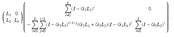
Denote  ,
,  ,
,  ,
,  ,
,  ,
,  ,
,  ,
,  ,
,  ,
,  . Then
  ,
,  , and
, and  , where
![$$\begin{aligned} M = \left[ \begin{array}{cc} M_1 &{}0 \\ M_2 &{} M_3 \end{array} \right] , \;\; \text {so that} \quad K M = \underbrace{ \left[ \begin{array}{cc} K_1 &{}0 \\ K_2 &{} K_3 \end{array} \right] }_{K} \left[ \begin{array}{cc} M_1 &{}0 \\ M_2 &{} M_3 \end{array} \right] = \left[ \begin{array}{cc} K_1 M_1 &{}0 \\ K_2 M_1 + K_3 M_2 &{} K_3 M_3 \end{array} \right] \nonumber \end{aligned}$$](/wp-content/uploads/2016/09/A352940_1_En_9_Chapter_Equ20.gif) and
and
![$$\begin{aligned} (I + K M)^{-1} = \left[ \begin{array}{cc} (I + K_1 M_1)^{-1} &{}0 \\ - (I + K_3 M_3)^{-1} (K_2 M_1 + K_3 M_2) (I + K_1 M_1)^{-1} &{} (I + K_3 M_3)^{-1} \end{array} \right] \nonumber \end{aligned}$$](/wp-content/uploads/2016/09/A352940_1_En_9_Chapter_Equ21.gif) so from (4.60) the projection operator for the feedback case (
so from (4.60) the projection operator for the feedback case ( ) is
) is
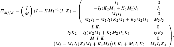 By reordering inputs and outputs, this can be partitioned by
![$$\begin{aligned} \left[ \begin{array}{cc} \varPi _{\bar{M}_1//\bar{K}_1} &{}0 \\ \varPi _{\bar{M}_2//\bar{K}_2} &{}\varPi _{\bar{M}_3//\bar{K}_3} \end{array} \right] \;\; \text {where} \;\; \varPi _{\bar{M}_1//\bar{K}_1}&= \bigg ( \begin{array}{c} I \\ M_1 \end{array} \bigg ) I_1 (I, K_1), \;\; \nonumber \\ \varPi _{\bar{M}_3//\bar{K}_3}&= \bigg ( \begin{array}{c} I \\ M_3 \end{array} \bigg ) I_3 (I, K_3) \end{aligned}$$](/wp-content/uploads/2016/09/A352940_1_En_9_Chapter_Equ7.gif)
are the projection operators for ![$$[\bar{M}_1,\bar{K}_1]$$](/wp-content/uploads/2016/09/A352940_1_En_9_Chapter_IEq58.gif) ,
, ![$$[\bar{M}_3,\bar{K}_3]$$](/wp-content/uploads/2016/09/A352940_1_En_9_Chapter_IEq59.gif) alone, and
alone, and
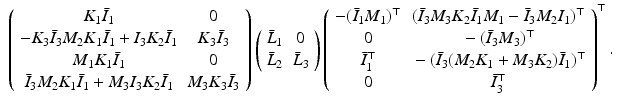
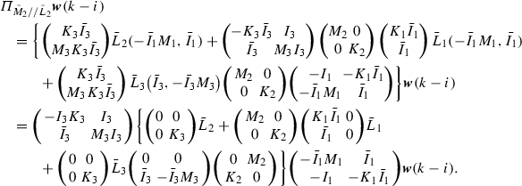
![$$\begin{aligned} \varPi _{\bar{M}_2//\bar{K}_2}&=\left[ \begin{array}{cc} - I_3 (K_2 M_1 + K_3 M_2) I_1 &{}\;\; I_3 ( K_2 \bar{I}_1 - K_3 M_2 I_1 K_1 ) \\ ( \bar{I}_3 M_2 - M_3 I_3 K_2 M_1 ) I_1 &{}\;\; \bar{I}_3 M_2 I_1 K_1 + M_3 I_3 K_2 \bar{I}_1 \end{array} \right] \nonumber \\&= \left( \begin{array}{cc} - I_3 K_3 &{}I_3 \\ \bar{I}_3 &{}M_3 I_3 \end{array} \right) \left( \begin{array}{cc} M_2 &{}0 \\ 0 &{}K_2 \end{array} \right) \left( \begin{array}{cc} I_1 &{}I_1 K_1 \\ - M_1 I_1 &{}\bar{I}_1 \end{array} \right) . \end{aligned}$$](/wp-content/uploads/2016/09/A352940_1_En_9_Chapter_Equ8.gif)
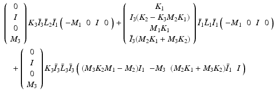
Next consider the inclusion of ILC, with associated component of (4.50) given by:
Using the identity  where
where  ,
,  ,
, 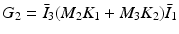 , we can denote
 which equals
 Using this, (9.9) can then be written as
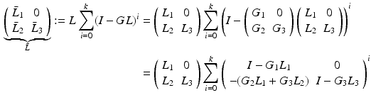
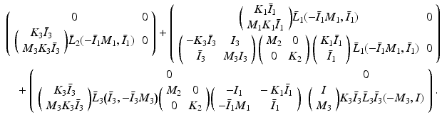
 By sequentially setting paired
  components to zero, this can be expressed as
Applying the same partitioning as in (9.12), (9.10) equals
 Recall that
  ,
,  ,
,
Comparison with (9.9), and using (9.7), means that we can write
![$$\begin{aligned} \varPi _{\bar{M}//\bar{C}} \varvec{w}(k+1) = \underbrace{ \left[ \begin{array}{cc} \varPi _{\bar{M}_1//\bar{K}_1} &{}0 \\ \varPi _{\bar{M}_2//\bar{K}_2} &{}\varPi _{\bar{M}_3//\bar{K}_3} \end{array} \right] }_{\varPi _{\bar{M}//\bar{K}}} \varvec{w}(k+1) + \underbrace{ \left[ \begin{array}{cc} \varPi _{\bar{M}_1//\bar{L}_1} &{}0 \\ \varPi _{\bar{M}_2//\bar{L}_2} &{}\varPi _{\bar{M}_3//\bar{L}_3} \end{array} \right] }_{\varPi _{\bar{M}//\bar{L}}} \varvec{w}(k-i) \end{aligned}$$](/wp-content/uploads/2016/09/A352940_1_En_9_Chapter_Equ12.gif)
where  ,
,  are the projection operators for
 ![$$[\bar{M}_1,\bar{C}_1]$$](/wp-content/uploads/2016/09/A352940_1_En_9_Chapter_IEq69.gif) ,
, ![$$[\bar{M}_3,\bar{C}_3]$$](/wp-content/uploads/2016/09/A352940_1_En_9_Chapter_IEq70.gif) alone, and
alone, and
To bound  we follow the proof of Theorem 4.6, with the relation
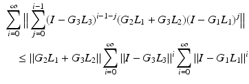
and summing each component of (9.13) we arrive at
Hence from (9.12)
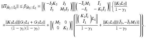
![$$\begin{aligned}\nonumber&\Vert \varPi _{\bar{M}//\bar{C}} \Vert \le \beta _{\bar{M}//\bar{C}} = \left\| \left[ \begin{array}{cc} \beta _{\bar{M}_1//\bar{C}_1} &{}0 \\ \beta _{\bar{M}_2//\bar{C}_2} &{} \beta _{\bar{M}_3//\bar{C}_3} \end{array} \right] \right\| \;\; \text {where} \;\; \beta _{\bar{M}_j//\bar{C}_j} = \beta _{\bar{M}_j//\bar{K}_j} + \beta _{\bar{M}_j//\bar{L}_j}, \nonumber \end{aligned}$$](/wp-content/uploads/2016/09/A352940_1_En_9_Chapter_Equ26.gif) with
with 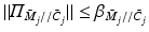 ,
,  . Adding bounds on (9.8) and (9.15) gives (9.6). Since
 ![$$[M_i |_{\varvec{z}(k)}, K_i]$$](/wp-content/uploads/2016/09/A352940_1_En_9_Chapter_IEq74.gif) is independent of plant dynamics
is independent of plant dynamics  ,
,  , then nominal closed-loop properties
  ,
,  are preserved.
, , , , , , , , , . Then , , and , where) is(9.7)
, alone, and(9.8)
(9.9)
where , , , we can denote components to zero, this can be expressed as(9.10)
, ,(9.11)
(9.12)
, are the projection operators for , alone, and(9.13)
we follow the proof of Theorem 4.6, with the relation(9.14)
(9.15)
, . Adding bounds on (9.8) and (9.15) gives (9.6). Since is independent of plant dynamics , , then nominal closed-loop properties , are preserved. Theorem 9 shows that a robust stability margin exists if  ,
,  are designed to minimise
  ,
,  ,
,  are designed to minimise
  , and
, and  ,
,  ,
,  ,
,  are stable operators. In particular, condition (9.5) reveals the dual aims of the designer:
Get Clinical Tree app for offline access
, are designed to minimise , , are designed to minimise , and , , , are stable operators. In particular, condition (9.5) reveals the dual aims of the designer:
Modeling: Include as accurate an interaction term as possible (thereby reducing the left hand side of (9.5)). This means that the lumped parameter global model of the upper arm,
  , must include enough joints associated with the array(s) to capture the main interaction effects.
Control: Following linearization, design feedback and ILC operators for the array and upper arm independently, minimizing and
and  respectively. Following this, design the interaction operators
  to minimize the gain bound
  associated with the interaction dynamics (and hence maximize the right hand side of (9.5)). The simplest approach is to set
  , which reduces bound (9.6) to