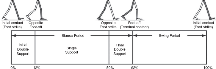
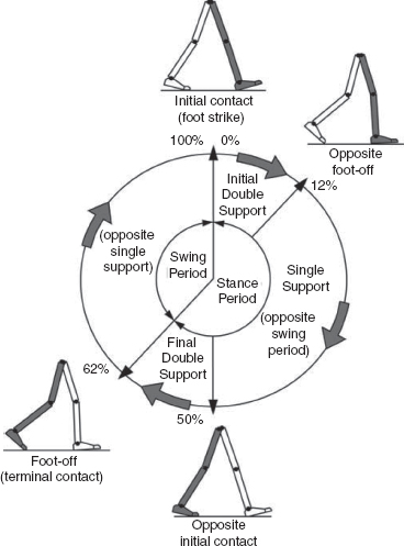
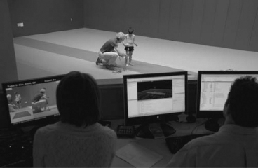
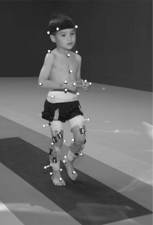
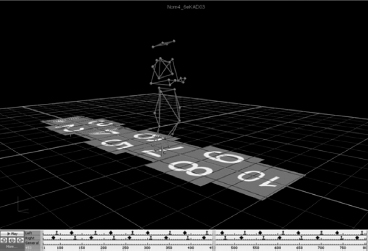
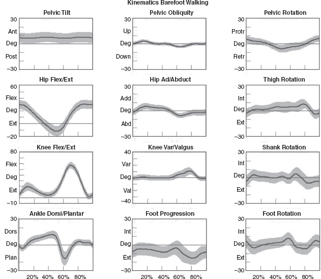
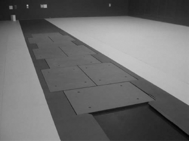
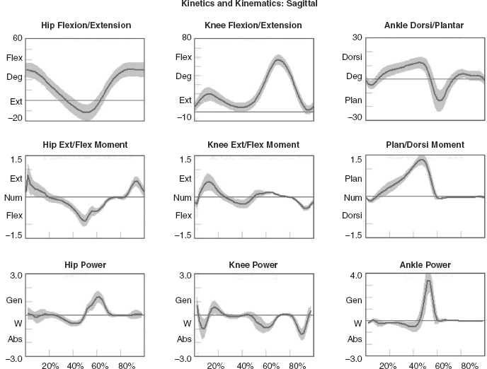
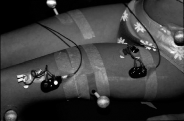
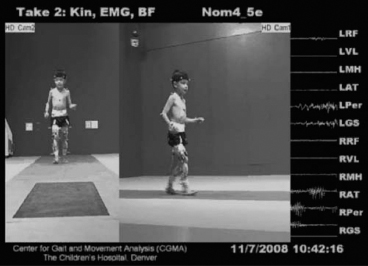
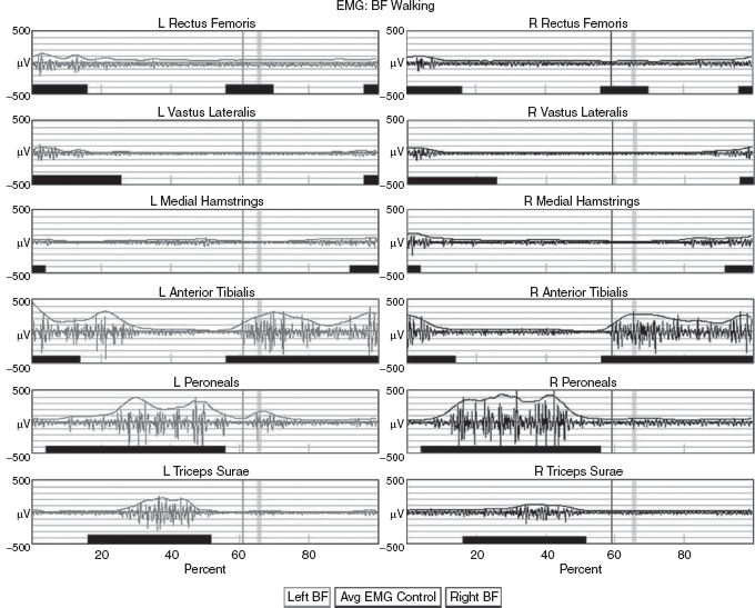
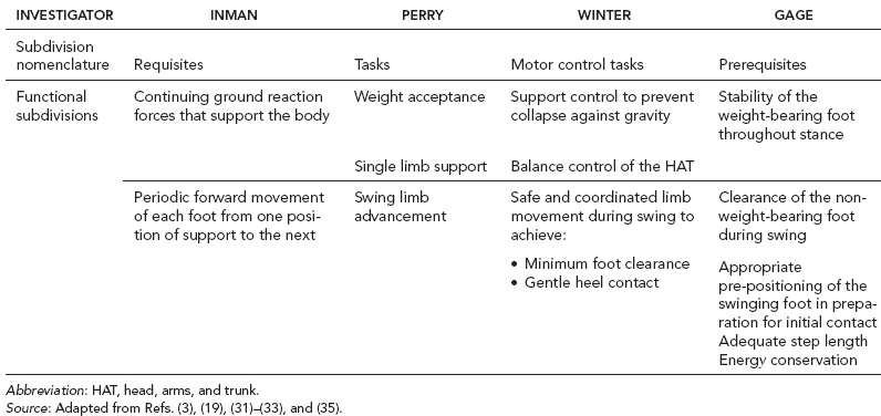
Quantitative Assessment of Gait: A Systematic Approach

QUANTITATIVE ASSESSMENT OF GAIT: A SYSTEMATIC APPROACH

James J. Carollo and Dennis J. Matthews

Bipedal walking is a distinctive and uniquely human behavior that is celebrated in childhood and cherished across the life span. In the words of Dr. Aftab Patla, a renowned motor control expert who had a long and distinguished career at the University of Waterloo, “… nothing epitomizes a level of independence and our perception of a good quality of life more than the ability to travel independently under our own power from one place to another.” Limitations in independent walking related to childhood disorders restrict education and employment options and access to social and cultural opportunities. Furthermore, a decline in walking ability directly affects the level of physical fitness so critical for health and well-being as we grow older, and contributes to a more sedentary lifestyle as an adult. Recent studies have linked habitual sedentary behavior to increased functional impairment and chronic disease risk in individuals with disability (1). This in turn can begin a cascade of chronic health issues and secondary conditions that can easily spiral out of control. Achieving and sustaining a functional level of walking ability is of the utmost importance to individuals with congenital or pediatric conditions and their families, and has a direct impact on their overall health status over their lifetime. Consequently, pediatric rehabilitation providers must be skilled in assessing walking and movement ability, and be comfortable utilizing all tools and techniques available to them to best manage their patients’ care and expectations related to this most basic human function.

Over the last 25 years, instrumented gait analysis (IGA) has become more commonplace, evolving into an accepted, objective evaluation that can guide surgical and rehabilitation therapy planning for the child with personal mobility challenges. IGA provides a quantitative and comprehensive snapshot of one’s characteristic movement pattern at a particular point in an individual’s development or at discrete intervals in his or her treatment. Clinicians can use this information to describe the complex physiologic interactions that lead to abnormal movement and motor control, and better understand their impact on gait, movement, and other functional activities.

Observational gait analysis is a common topic during residency and most pediatric physiatrists are familiar with the procedures. However, training in the use of quantitative tools common to IGA and available from a modern clinical motion laboratory are frequently overlooked in postgraduate education, with the inclusion in the curriculum being highly dependent on the availability of such a facility during their training. Despite the advances in technology that have made IGA more commonplace in clinics around the world, only a handful of Physical Medicine & Rehabilitation (PM&R) residency programs are associated with motion analysis facilities. Even fewer are associated with clinical motion laboratories accredited by one of the two independent accreditation organizations, the Commission for Motion Laboratory Accreditation (CMLA) in North America, and the Clinical Movement Analysis Society (CMAS) of the United Kingdom and Ireland. Laboratories that have achieved accreditation conform to common standards of practice, quality, and information reporting that are the benchmark for IGA in clinical practice. This chapter can be used as a guide for those interested in utilizing data from accredited facilities in their practice regardless of their level of exposure to IGA in the past.

Mastery of IGA procedures along with the ability to perform meaningful interpretations that are clinically relevant remains challenging for many clinicians. We believe underutilization of modern gait analysis techniques in pediatric rehabilitation is related to the difficulty associating gait deviations seen in an IGA report with specific functional deficits during the walking cycle. Fundamental to making this connection is a clear understanding of the functional demands of normal gait. Armed with this understanding, the essential features of normal, efficient locomotion can be easily recognized, and this provides the basis for identifying the absence of these features in the child with gait dysfunction. When applied systematically, this evidence-based approach can provide a logical strategy for clinical gait analysis and the management of gait disorders (2).

Therefore, the goal of this chapter is to familiarize clinicians with fundamental gait analysis principles by focusing on the inherent functional requirements of normal locomotion. This provides a framework for using specific measurements from an IGA report to pinpoint the joint and/or muscle system responsible for a particular functional deficit, and the subsequent target for clinical intervention.

NORMAL GAIT IS CYCLICAL AND SYMMETRIC

The principal goal of locomotion is to efficiently propel the body forward. The most natural way for humans to accomplish this task is to employ a bipedal gait pattern, where the base of support alternates between legs. Inman has described the cyclical alteration of each leg’s support function and the existence of a transfer period when both feet are on the ground as essential features of normal locomotion (3). Since normal gait assumes no biomechanical advantage provided by either limb, a natural consequence of these essential features is the existence of a repeatable pattern that is both cyclical and symmetric. Figure 5.1 illustrates one complete gait cycle, or stride, and includes the time periods and temporal events associated with foot/floor contact that necessarily arise from changing the support limb. Temporal events are specific moments in time that divide the gait cycle into discrete time periods of finite duration, and are identified by the stick figures along the top of Figure 5.1. Typically, a cycle begins when one foot makes contact with the walking surface (initial contact) and ends when that same foot strikes again. This is the functional definition of a stride. Using such a convention allows a stride to be time-normalized, where a specific stride location is expressed as a percentage of the total cycle time or stride period. Time normalizing the gait cycle facilitates comparing subjects with different stride lengths, stride periods, and walking speeds on the same scale. Figure 5.1 illustrates the time periods and temporal events relative to the shaded ipsilateral side. If a subject’s gait pattern is normal, the stride would be inherently cyclical and symmetric, with equal time periods on each side. The temporal event of foot-off (sometimes referred to as terminal contact) separates the gait cycle into stance and swing periods. Typically, the stance period accounts for 60% to 62% of the total gait cycle and the swing period takes the remaining 40% to 38%. We have intentionally refrained from using the terms “stance phase” and “swing phase” here to avoid confusing these intervals with the phases of gait to be introduced in a later section, although in common practice, the terms can be used interchangeably.

The stance period includes two intervals of double limb support at the stance/swing transitions, each lasting approximately 10% to 12% of the gait cycle at typical walking speeds. These are generally described as initial and final double support, but can also be identified in the context of the leading limb as right or left double limb stance period. The duration of the double limb support periods decreases with increasing walking speed, reaching zero at the moment running begins. The time interval between the initial and double support periods is defined as the single support period, and is the same duration as the swing period of the opposite limb. Assuming normal symmetry, any reduction in double limb support time is associated with a proportional increase in single limb support time, but since single limb support always corresponds to the contralateral swing period, the overall stance period decreases, reaching 50% at the initiation of running when double limb support reaches zero. When both limbs’ primary temporal events of foot strike (initial contact) and foot-off (terminal contact) are represented on the same time scale, the duration of each time period is easily illustrated.

FIGURE 5.1 A typical gait cycle normalized in time, and represented on a linear scale from 0% to 100% of the total stride. This repeating cycle begins with initial contact and ends with the next initial contact of the same foot. The stick figures shown on top represent temporal events associated with foot-to-floor contact. They divide the cycle into swing and stance periods, one period of single support and two equal periods of double support.

These general terms for temporal events are applicable, regardless of gait pathology. Other terms are routinely used to identify temporal events marking the transition from the swing period to the stance period (heel strike, forefoot initial contact, foot-flat) and stance to swing (toe-off, push-off), but should only be used when they clearly describe the observed foot/floor contact pattern.

While period durations relative to a single side are easily described when the gait cycle is represented on a linear scale, left/right symmetry may be more easily conceptualized when the gait cycle is wrapped around a unit circle (2,4,5), as shown in Figure 5.2. For typically developing children and adults, ipsilateral and contralateral initial contact and foot-off will occur directly opposite each other around the circle, or 180 degrees out of phase. This graphically illustrates that the resulting time periods must be of equal duration for left and right single support, initial and final double support, and left and right swing periods. Any disruption in the natural sequence of temporal events anywhere along the cycle as a result of physical impairment, weakness, or spasticity will result in incorrect timing for the events that follow. This necessarily leads to a loss of symmetry that can be quantified by comparing the timing of temporal events between sides. Changes in symmetry reflected in the gait period durations are an index of gait pathology, and measuring this simple quantity can be quite useful for evaluating treatment performance over time.

FIGURE 5.2 A typical gait cycle normalized in time, but wrapped around a continuous unit circle to illustrate symmetric phase relationships of temporal events and time periods. The beginning and end of the cycle occur at the 12 o’clock position. The temporal events of initial contact and foot-off for each leg are typically opposite each other on the unit circle, and the single support period of one limb is equal to the swing period of the opposite limb.

Since the duration of the swing period combined with leg length determines the distance covered by the swinging limb, deviation from normal symmetry and timing will give rise to differences in step length on each side, and subsequently the total distance traveled per gait cycle. By definition, step length and stride length are not synonymous. Step length is the distance (in the direction of progression) from a point of ground contact of the trailing foot to the next occurrence of the same point of ground contact with the leading foot. It is measured during double support and named for the leading limb. In contrast, stride length is the distance from initial contact of one foot to the next initial contact of the same foot, corresponds directly to the stride period, and is equivalent to the sum of successive left and right step lengths. Recognizing that speed is defined as the ratio of distance per unit time, the quantities of step length, stride length, cadence (steps per minute), and walking speed are mathematically related by simple formulas:

2 steps = 1 stride

walking speed (m/s) = [cadence (steps/min) × stride length (m)]/120

stride length (m) = [walking speed (m/s) × 120]/cadence (steps/min)

step length (m) = [walking speed (m/s) × 60]/cadence (steps/min)

These basic outcome measures of overall gait performance, including the timing measures previously described and other quantities such as stance/swing ratio, are collectively known as temporal–distance or temporal–spatial parameters. They can provide considerable insight into the functional consequence of subtle gait abnormalities on walking performance. For example, children with cerebral palsy (CP) may experience foot clearance problems during limb advancement due to excessive ankle plantar flexion and/or decreased knee flexion during swing period. Evidence of this could be found in prolonged single support times on the more normal or less involved side (a consequence of the longer swing time on the more involved side), and a reduced stance period, step length, and stance/swing ratio on the more involved side (6). If the source of the limb advancement problem can be attributed solely to the excess plantar flexion, the simplest intervention would be to prescribe a solid or posterior leaf-spring ankle foot orthosis (AFO) with a rigid plantar flexion stop to restrict excess plantar flexion during swing. Evidence that this intervention improved gait performance could be found in more symmetric single limb support times and step lengths, a more normal stance/swing ratio, and a higher walking speed.

While clinical motion laboratories routinely compare a patient’s temporal–spatial measures to age-matched normative values, caution should be used when interpreting these results. Temporal–spatial parameters of cadence and stride length are directly related to walking speed (7), and since humans routinely walk at a variety of speeds, simple deviations from reference values alone may not be indicative of gait pathology. Rather, reduced values for these measures may simply reflect the need to adopt a speed appropriate to the terrain, the required task, or the size of the room (8). A person’s natural gait is also dependent on the environment, with studies showing that subjects walk faster on a long walkway compared to a short one, and typically walk faster in outdoor studies compared to indoor studies (9). This lack of consensus regarding normal values supports the convention adopted by most clinical laboratories to compare patient results to their own laboratory-collected references, where these environmental factors can be consistent for all subjects. Nevertheless, while it is “normal” to walk at a variety of speeds, it clearly is abnormal to walk asymmetrically, so side-by-side differences in temporal–spatial measures within a particular patient should always be investigated.

When comparing temporal–spatial parameters in children, even greater care must be exercised, since several age-related differences arise from the close relationship of these measures to leg length and gait maturity (10). Sutherland has shown that in typically developing children, heel-first initial contact, sagittal plane knee flexion wave, reciprocal arm swing, and an adult joint angle pattern are acquired prior to the development of mature temporal–spatial parameters (11). All of these adult gait characteristics arise before the age of 3 years in most children (6). Because of this, Sutherland believes that gait maturity is best judged by the following five features, which he calls “determinants of mature gait” (11). These are: duration of single support, walking speed, cadence, step length, and ratio of pelvic span to ankle spread (P/A ratio). Notice that in addition to the first four measures that are fundamental temporal–spatial parameters, an anthropometric measure (P/A ratio) has been added, mainly to address the increased hip abduction and wider base of support common in the immature child’s gait. In general, walking speed, step length, single support, and P/A ratio increase linearly with advancing age, with the greatest changes occurring during the first 4 years of life (6). Cadence decreases significantly between the ages of 1 and 2 years, after which it gradually continues to decrease (10). By age 4, the interrelationship between temporal and distance measures is fixed, although stride length and walking speed continue to increase with increasing leg length. Muscle phasic alterations in the early walkers are generally characterized by prolonged activation periods and subsequent longer periods of agonist/antagonist cocontraction around the joints of the lower extremities (12), most likely caused by neurologic immaturity associated with incomplete myelination (6). Despite these age-related differences that continue until skeletal maturity, the fundamental features and temporal–spatial parameter interrelationships associated with a normal, repetitive gait cycle are in place by age 4. For this reason, asymmetry detected using temporal–spatial measures can be used as indicators of gait pathology in both children and adults.

Because normal gait should be cyclical and symmetric, the existence of even small amounts of step-to-step variability may be an indication of gait pathology. Gait is most variable in the toddler, but gradually stabilizes as the child reaches adolescence (9). Hausdorff and colleagues have shown that the coefficient of variation for stride time in typically developing 3- to 4-year olds is approximately 6%, but decreases to 2% in 11- to 14-year olds (13). In older adults, increased variability is associated with increased risk of falling, with speed variability the single best predictor of falls (9). These examples provide further evidence of the importance of a cyclical and symmetric gait pattern and how variations in symmetry and cycle times reflected in the temporal–spatial parameters of gait may be associated with gait pathology.

TYPICAL COMPONENTS OF AN INSTRUMENTED GAIT ANALYSIS

As mentioned in the introduction, the phrase instrumented gait analysis (IGA) is often used to describe the application of computerized measurement technology to clinical gait analysis for the purpose of enhancing the interpretive power of the analysis beyond what can be discerned using observational and physical examination methods alone. The specialized nature of the systems used to perform an IGA typically requires a dedicated motion laboratory with specialists from clinical and technical disciplines to guide the patient through the testing procedures, make the required physical and anthropometric measurements, and capture and process all data (Figure 5.3). Analyses typically require 1.5 to 2 hours of patient contact time and between 8 and 12 hours of processing and analysis time, depending on the complexity of the patient referral and the number of measurements required to answer the clinical question. It is not within the scope of this discussion to comprehensively describe the full set of measurement tools available for clinical gait analysis in children. For this, the reader is referred to several excellent descriptions that are widely available (5,14–20). However, since it is important for the discussions that follow, we will briefly introduce the primary measures used, some tips for their practical application, and give examples of typical recordings as a reference.

FIGURE 5.3 A motion laboratory clinical specialist works to place reflective markers on a subject while the technical staff prepares for data capture.

In addition to the temporal–spatial parameters described in the last section, the primary measurements comprising IGA are gait kinematics, kinetics, and dynamic electromyography (d-EMG) (16). While there are certainly additional areas of measurement and many useful instruments that can be included in a comprehensive IGA, these three measurement categories are commonly accepted as the minimum necessary for clinical evaluation of the patient with gait dysfunction. They have also been identified as a specific requirement for accreditation by the CMLA and the CMAS of the United Kingdom and Ireland (21).

Gait kinematics is a general term that refers to measurement of the linear and angular displacements, velocities, and accelerations of body segments throughout the gait cycle. Generally expressed in terms of the joint angles between each limb segment, these quantities are most often described three-dimensionally using anatomical planes relative to the more proximal segment, but also includes the global position of the pelvis (pelvic tilt, obliquity, and rotation) and foot (foot progression angle) relative to a fixed laboratory coordinate system typically located in the middle of the walkway. Modern kinematic analysis systems use an assortment of markers or targets that are attached to the subject at strategic locations and can be tracked by specialized cameras or electromagnetic detectors (Figure 5.4). The kinematic measurement system identifies the position of the targets from multiple perspectives in three-dimensional (3D) space using a high sampling rate (>100 Hz) as the subject walks through a calibrated measurement volume. This determines a unique trajectory for each target, which can then be reconstructed by the computer utilizing a kinematic limb-segment model to produce a 3D animation of the walking subject within the virtual environment of the computer display (Figure 5.5). From this mathematical representation of the subject, kinematic graphs and interactive reports can be produced to facilitate the clinical analysis of the child’s gait pattern.

FIGURE 5.4 Subject with reflective markers or targets placed at strategic anatomic locations walks through a modern motion analysis laboratory. The location of the targets depends on the mathematical requirements of the limb-segment model used to calculate the kinematic values needed for analysis. This subject is using a full body marker set based on the Conventional Gait Model.

Kinematic measurement systems rely heavily on motion-capture technology and specialized software that, fortunately, have found a major market in the video game and motion picture industry. This has had the positive effect of substantially lowering the startup cost of these systems in recent years, making the technology more available to the clinical community and improving the accuracy, precision, camera resolution, and processing speed. These advances have also increased the complexity of the kinematic models that can be implemented, which offers the promise of more comprehensive and anatomically correct descriptions of motion. However, it may also introduce new challenges since increased model complexity necessitates greater software complexity. Furthermore, the requirement for model validation with each new software release necessitates regular laboratory procedural changes, and may introduce data discrepancies when patient results are compared over time using different models. Recognizing these potential technical concerns, gait kinematics represent an integral component of clinical movement analysis and are essential for analyzing the child with gait dysfunction. Figure 5.6 shows a set of 3D kinematic graphs associated with a sample of typically developing 12 to 13-year-old subjects used as a normal reference in our laboratory. We will discuss these kinematic graphs in more detail when discussing critical events in a later section.

FIGURE 5.5 Three-dimensional animation of the walking subject within the virtual environment of a computer display.

While measurements of gait kinematics provide a quantitative description of body segment and joint movement during walking, gait kinetics describe the forces that cause these movements and the calculated quantities that arise when a subject’s reaction forces and 3D kinematics are applied to a mathematical model of the body. Since joint and muscle forces cannot be measured directly from the walking subject, the forces due to foot/floor contact are measured using a specialized instrument known as a force platform embedded in the walkway. The force platform measures the vertical, fore–aft shear, and medial–lateral shear components of the ground reaction force (GRF), which is the force vector acting at the supporting surface that is equal and opposite to the sum of all muscular, gravitational, and inertial forces generated by the body in motion. Since a force platform measures the magnitude and direction of the GRF as a single resultant vector quantity, only one foot can be in contact with the platform at a time for a valid measurement. In order to measure multiple foot strikes from both feet, the subject either needs to walk multiple times across a single platform or the laboratory needs to include a force platform array with multiple platforms in different orientations so that several clean foot strikes from both sides can be recorded in as few a number of passes as possible. A larger force platform array reduces alterations of gait characteristics in children with neuromuscular diseases in several ways. Installing multiple force platforms into the walkway reduces the number of trials required and thus minimizes the risk of fatigue. Furthermore, having multiple force platforms lessens the possibility of “targeting,” which will alter the subject’s characteristic gait pattern. Figure 5.7 shows the large 10-platform array of 60 cm × 40 cm force platforms currently used in our laboratory, and illustrates how sequentially rotating the long axis of each platform 90 degrees can accommodate a wide variety of stride lengths and step patterns for children and adults.

FIGURE 5.6 Normal three-dimensional kinematic graphs constructed using a sample of typically developing 12- to 13-year-old subjects. These data are used as a reference for comparing kinematic data from clinical subjects of the same age. The dark line is the average of all subjects and the gray band represents ± one standard deviation.

FIGURE 5.7 Large 10-platform array of 60 cm × 40 cm force platforms used in The Center for Gait and Movement Analysis at Children’s Hospital Colorado in Aurora, Colorado. The “hopscotch” pattern of the platform array permits the recording of several individual foot strikes from both feet in a single walking pass. For illustration purposes, each platform is shown without its protective floor covering, which caused the platforms to blend into the surrounding walkway when applied.

The direct measurement of the individual force components and the vector sum of the GRFs has historically been used to evaluate gait kinetics and facilitate a more qualitative pre-/postsurgical comparison. The most useful clinical application of gait kinetics, however, is when it is combined with GRF measurement and a kinetic model of the lower extremities to calculate joint kinetics, specifically joint moments and powers (22). The most common way to accomplish this is to apply an “inverse dynamics” model of the lower extremity using the anthropometric dimensions of each segment (typically seven segments, including the pelvis and both thighs, shanks, and feet) and estimates of each segment’s center of mass (COM) and inertial quantities. The forces at each joint can then be solved sequentially, starting from the GRF at the floor and working proximally, using the linear and angular forms of Newton’s second law:

Linear: force = mass × acceleration (F = ma); angular: joint moment = moment of inertia x angular acceleration (M = Ia).

By convention, joint moments can be considered either external or internal. External moments reflect the forces, acting on the body through the skeleton, that arise from the GRF, and since they reflect an external biomechanical load, are sometimes called demand moments. Internal moments describe the force generated by the muscles and ligaments acting on the skeleton to balance the external moments, and because they are counteracting an external load, are sometimes called response moments. Aside from their different functional descriptions, external and internal moments for the same joint are of equal magnitude and differ only in their mathematical sign. The joint moments described in a typical IGA report are internal moments, but this should always be confirmed since the sign and direction of the curves will be reversed if they actually describe external moments. Joint moments are vector quantities that describe the net torque around each joint but do not provide the individual force contribution from each agonist/antagonist pair or from individual muscles. Nevertheless, the net moment around the joint is quite useful because the magnitude and sign of the curve at any instance in the cycle can illustrate if one half of the agonist or antagonist pair is dominating at a specific point in the gait cycle. Net moment values can aid in clinical interpretation of gait by comparing them to reference values for typically developing children and by observing changes in the values before and after treatment. In addition, net moment values are helpful in understanding how a child may be compensating at a given joint for weakness or limited range of motion (ROM) at an adjacent joint. Figure 5.8 shows the sagittal plane kinematics, sagittal plane joint moments, and total joint power for the hip, knee, and ankle from a sample of typically developing 12 to 13-year-old subjects that we use as a normal reference.

FIGURE 5.8 Graphs of sagittal plane kinematics, sagittal plane joint moments, and total joint power for the hip, knee, and ankle constructed using a sample of typically developing 12- to 13-year-old subjects. These data are used as a reference for comparing kinetic data from clinical subjects of the same age. The dark line is the average of all subjects and the gray band represents ± one standard deviation.

Once the 3D moments at each joint have been calculated, joint power at any time in the gait cycle is the product of the joint moment and the corresponding angular velocity (instantaneous slope of the joint angular displacement curve from kinematics) at each percent interval of the gait cycle:

joint power = joint moment × joint angular velocity
P(t) = M(t) × ω(t)

Electromyography (EMG) is an important tool for evaluation of muscle and neurologic function and is well understood by the pediatric physiatrist. When used in the context of IGA, the purpose is slightly different from the conventional application. The primary objective of EMG in clinical gait analysis is to identify periods of muscle activation during walking so that decisions can be made regarding the appropriateness of muscle timing for agonist pairs as they selectively activate and deactivate during the gait cycle. This is the reason that we refer to this as dynamic electromyography or d-EMG, since the focus is on the phasic response of muscle during walking or some other functional activity. Since the subject will not be in a stationary position for the test, the instruments and technical procedures are also different from conventional diagnostic EMG. d-EMG requires a bipolar arrangement of electrodes and miniature differential amplifiers with a high common mode rejection ratio (CMRR) placed close to the site of the recording to ensure the EMG signal is not overwhelmed by motion artifact while the subject moves (Figure 5.9). Differential amplifiers with high CMRR (typically greater than 90) amplify voltage differences between the inputs and reject common voltages that may arise from movement of the electrodes or the soft tissue vibration that occurs with foot contact. Surface electrodes are the most commonly used electrode type for recording d-EMG from the pediatric patient to avoid the emotional trauma and change in gait pattern that indwelling electrodes often cause. Typically, the active portion of each electrode in the bipolar pair should be small and the pair should be placed as close together as possible along the long axis of the muscle (≤1 cm diameter, ≤2 cm separation) to minimize the effect of crosstalk from surrounding muscles. Unfortunately, surface electrodes are only suitable for recording muscle groups that are directly subcutaneous; if there is a need to evaluate deeper muscles individually, fine-wire electrodes made of a bipolar pair of 50-micron platinum wire must be inserted directly into the muscle of interest using a 25- to 28-gauge needle. When required, this is the most invasive aspect of an IGA, and should be used only when necessary in the pediatric patient and after all other data have been collected, since the level of patient cooperation and the likelihood of a typical gait pattern decrease considerably after a needle stick. In practice, most of the muscles of interest to the pediatric physiatrist can be successfully recorded using the surface electrode approach if proper procedures to minimize crosstalk and reduce motion artifact are followed.

FIGURE 5.9 Patient with bipolar surface electrodes and small instrumentation amplifiers for recording dynamic EMG while he or she walks. This illustrates the electrode placement for the left vastus lateralis (distal location) and left rectus femoris (proximal location). Each electrode is connected to an instrumented backpack and then hardwired to the recording instruments. A wireless EMG recording system using similar electrodes but with individual transmitters for each muscle is shown in Figure 5.4.

Before the EMG recording can be used for clinical interpretation, the raw data must be filtered, processed, and time-normalized so that periods of muscle activation during the gait cycle can be identified. A good reference for processing guidelines is available from the International Society of Electrophysiology and Kinesiology, where they state that surface electrode recordings should be bandpass-filtered between 10 Hz and 350 Hz and fine-wire recordings filtered between 10 Hz and 450 Hz. This maximizes the signal, minimizes the noise, and reduces motion artifact. In modern systems, the filtered EMG data are sampled by analog-to-digital converters. Further processing is performed by computer using specialized software or in concert with the motion-capture system. Data can be presented as a continuous recording of “raw” EMG, an ensemble average of several cycles of EMG normalized to the gait cycle, or as linear envelopes reflecting the EMG magnitude throughout the gait cycle after rectification and integration of the raw EMG signal. In our laboratory, we have developed a system to superimpose the EMG signal over the observational video recording of the walking subject to screen for faulty EMG recording during the analysis and to better understand the interaction between observed movement and muscle activation (see Figure 5.10, right side). Regardless of how these data are presented, the goal is to use the EMG recording to identify periods of abnormal muscle activity and determine if this activity is responsible for abnormal movement patterns presented by the patient. Typically, the patient’s activity is compared to a normal EMG reference, and deviations from normal values are scrutinized for their contribution to the overall movement pattern. Figure 5.11 shows filtered and time-normalized EMG for 12 muscles of the lower extremity from a 15-year-old typically developing subject used as a laboratory reference, along with published normal EMG activations represented as solid black bars at the bottom of each graph. The high-magnitude sections of the EMG recording for each muscle correspond to the published normal values, confirming that this typically developing subject has a normal adult activation pattern.

FIGURE 5.10 Biplane high-definition video recording with superimposed real-time EMG traces of six muscles bilaterally from a typically developing subject used as a reference at CGMA. The raw, unfiltered EMG recording provides immediate feedback on the quality of the EMG signal and the synchronization of muscle activity with observed movement.

When EMG recordings are combined with kinematics, kinetics, temporal–spatial parameters, radiographs, and physical examination results, a comprehensive snapshot of the subject’s walking pattern is revealed, providing an empirical basis for identifying the functional cause of a gait abnormality. However, to use these data successfully, we must return to the normal gait cycle to understand the functional requirements for walking, since these requirements are a natural consequence of subdividing the cycle on the basis of function.

IMPAIRMENT IDENTIFICATION IS FACILITATED BY SUBDIVIDING THE GAIT CYCLE

While a repetitive gait cycle arises from the alternating base of support used by all bipeds, the existence of this cycle provides great opportunity for clinical and biomechanical analysis of a child with gait dysfunction. In particular, a repetitive cycle lends itself to natural subdivision, which in turn, leads to a sequence of events that must be performed in order and with the correct timing for efficient walking to occur. The earlier section titled “Normal Gait Is Cyclical and Symmetric” discussed temporal subdivisions of the gait cycle delineated by foot/floor contact and their use in comparing limb symmetry, measuring outcomes, and the general characterization of overall gait performance. The focus of the current section is to describe another type of gait-cycle deconstruction, one based on functional subdivisions. For this approach, the functional prerequisites of walking are identified, providing a framework for subdividing the gait cycle into functional divisions (24). It is then possible to use the measurements available from IGA to identify quantitative differences at each joint and the specific functional abnormalities that occur at critical moments in the gait cycle (25,26).

FUNCTIONAL PREREQUISITES FOR WALKING

In their landmark paper published in 1953, Saunders, Inman, and Eberhart (27) described six gait subdivisions that they referred to as the “determinants” of normal gait. This treatise was significant in that it was perhaps the first formalized delineation of the gait cycle that explained how coordinated movements of the hip, knee, and ankle at specific points in the cycle led to efficient forward progression. Each determinant’s influence on the 3D path of the whole-body COM was described using simple theoretical models, and the cumulative effect of all six determinants led to a smooth, low-amplitude trajectory that was assumed to be consistent with optimal, efficient locomotion. Specifically, Inman and colleagues believed that minimizing vertical and horizontal motion of the COM would maximize walking efficiency, since unnecessarily raising and lowering the COM would be wasteful from a potential energy perspective. By changing functional limb length with the addition of joints to an initially jointless model of the lower extremities and pelvis, each determinant served to smooth different portions of the COM trajectory, effectively raising the COM during double support and lowering it during single support. While it is true that unnecessarily large and abrupt movements of the COM reduce gait efficiency, some of the specific determinants identified by Inman and colleagues have now been discredited (28–30). The improved accuracy and temporal resolution of kinematic measurement instruments over the last 50 years have uncovered problems with the timing of some of the theoretical mechanisms described in the original paper, and in the case of longer step lengths, larger COM displacements are not necessarily associated with decreased gait efficiency.

While the relevance of specific determinants may now be in dispute, the real impact of this work is that it inspired generations of investigators to consider biomechanical explanations for gait dysfunction and led a few students of Dr. Inman to develop clinically applicable gait-cycle decompositions derived from the functional requirements of walking. In a later monograph (3), Inman described two basic functional requisites of walking that he deemed necessary for any form of bipedal gait, no matter how distorted by physical disability or assisted by prosthetic or orthotic devices. These are (a) continuing GRFs that support the body and (b) periodic forward movement of each foot from one position of support to the next.

FIGURE 5.11 Filtered and time-normalized EMG for 12 muscles of the lower extremity from a typically developing 15-year-old subject. The black bars at the bottom of each graph are constructed from published normal EMG activations and are used as reference values. The smooth curve above the EMG activation is a processed EMG signal obtained by rectifying and integrating the raw EMG. Notice that each EMG activation pattern above a baseline level is contained within the reference bar indicating a normal EMG pattern. In this typically developing subject, there is very little EMG activity from the rectus femoris during initial swing.

These essential features of walking give rise to a periodic gait cycle that must always be present for continued locomotion. An orthopedic resident of Dr. Inman, Jacquelin Perry, recognized that the physical demands of supporting the body against gravity varied, depending on whether the stance limb was accepting the initial impact or continuing to carry the weight of the body during single support. To address this, she developed the notion of three functional gait tasks (31): weight acceptance, single limb support, and swing limb advancement. Dr. Perry considered weight acceptance the most demanding of the three functional gait tasks since it requires the stance limb’s musculature and bony and ligamentous structure to provide shock absorption, initial limb stability (stiffness), and maintenance of forward progression. Preparation for the demands of weight acceptance begins late in the swing period, when pre-positioning of the leading limb occurs to correctly align the foot to accept weight at initial contact. The physical demands are lower for the task of single limb support, despite the fact that one leg alone has the complete responsibility for supporting body weight, maintaining whole-body stability (balance), and restraining forward momentum. This reduced physical demand during the task of single limb support is due to the inherent passive stability provided by the knee ligamentous structure and the force balance at the hip as body weight moves forward (31). An essential functional requirement for this task is strong eccentric contraction of the calf musculature to control the tibia (and subsequently the rest of the stance limb) as it rotates over the fixed base of support provided by the foot. When the task of single limb support ends and swing limb advancement begins, the physical demands increase once again, since the three goals of weight transfer, limb advancement, and foot clearance must all be accomplished. Similar to the weight acceptance task, important preparatory actions must begin before the swinging limb is lifted from the supporting surface at the end of the stance period to meet the functional demands of swing limb advancement.

Findings from other investigators support the existence of these three fundamental gait tasks, although each investigator has used a somewhat different terminology when describing them (Table 5.1). Winter has characterized walking as an extremely complex motor control task that requires three elements: support control to prevent collapse against gravity (32); balance control of the head, arms, and trunk (HAT) acting as an inverted pendulum (33); and safe and coordinated lower limb movement during swing for minimum foot clearance and gentle heel contact (19). Dr. Winter and colleagues have also stated that the goals of these tasks can still be accomplished after disease, injury, or loss of function because of the inherent redundancy of lower extremity musculature and rapid adaptability of the central nervous system (34). It is interesting that Perry and Winter have identified essentially the same three gait tasks, despite approaching the study of gait from two different perspectives: clinical analysis of pathologic gait and biomechanics of human movement, respectively. This lends support to the existence of these three elements and warrants using them to understand functional deficits in subjects with gait pathology.

Gage has expanded on this description by identifying five elements essential to walking that he has referred to as “priorities” or “prerequisites” of normal gait (35). This functional subdivision of the gait cycle encompasses the three tasks described previously, but adds swing period elements necessary to ensure appropriate weight acceptance and the global task of energy conservation. In the order of functional priority, these are stability of the weight-bearing foot throughout stance, clearance of the non-weight-bearing foot during swing, appropriate pre-positioning of the swinging foot in preparation for initial contact, adequate step length, and energy conservation. This prioritization is influenced by Dr. Gage’s interest in the gait of children with CP, and includes a gait efficiency task (energy conservation) to address the reduced functional capacity or endurance of many individuals with pathologic gait. He also identifies several physiologic and biomechanical mechanisms common to normal gait that can improve energy conservation. These are eccentric muscle contraction, return of “stretch energy” from prestretched muscles immediately prior to concentric contraction, biarticulate muscles functioning as energy transfer straps, and joint passive stability from the effects of GRFs whenever possible to spare muscle activation (36). While other investigators have addressed the functional prerequisites of gait (15,25,37), the contributions described previously form the basis of the strategy described in this chapter.

TABLE 5.1 FUNCTIONAL SUBDIVISIONS OF THE GAIT CYCLE ATTRIBUTED TO DIFFERENT INVESTIGATORS

PHASES OF THE GAIT CYCLE

Since the tasks of weight acceptance, single limb support, and swing limb advancement can only be accomplished successfully if appropriate limb movement patterns occur sequentially and with correct timing, Dr. Perry developed a systematic method of subdividing the gait cycle to simplify pattern identification and facilitate observational gait analysis (24). Now known as the Rancho classification, in honor of Rancho Los Amigos Medical Center where Dr. Perry and colleagues of the Pathokinesiology Service developed this method, it relies on eight subdivisions of the gait cycle, referred to as phases of gait. While in general, both phases and periods refer to specific time slices around the gait-cycle unit circle, Perry prefers to use the term “phase” for intervals that have specific functional significance and have a clear relationship to the three identified gait tasks described in the previous section. The Rancho classification provides a framework for functionally organizing the gait cycle harmoniously with the three fundamental gait tasks, and after 30 years of refinement, this approach has proven to be a powerful tool for identifying specific functional deficits or gait impairments during each phase of gait. IGA can be used to quantify the magnitude of a functional deficit at a joint by reviewing the kinematic and kinetic data, or abnormal muscle timing by reviewing the EMG. This provides evidence and helps pinpoint the specific region or system most responsible for the overall gait abnormality, and suggests interventions to directly correct the identified functional deficit or gait impairment in each phase.

The eight phases described by Dr. Perry are identified in Table 5.2. Notice that all but the first phase (initial contact) represent separate time intervals between 0% and 100% of the gait cycle. Figure 5.12 illustrates the phases of gait in sequence around the unit circle, with stick figures signifying the temporal event delineating the beginning and end of each phase. Phases are shown equally spaced in this figure for clarity; typically, each phase will not be of the same time duration. Initial contact is considered a phase of gait since it marks an important transitional point between swing limb advancement and the challenging task of weight acceptance, although unlike the other phases, it is a single instant in time. The other important transitional period (from stance to swing) occurs during final double support and is known as the phase of preswing. In terms of temporal events, final double support (and therefore pre-swing) is considered part of the stance period because this interval ends with foot-off. However, in terms of gait phases, this interval also marks the first phase of the swing limb advancement task, highlighting the fact that from a functional standpoint, pre-swing has more to do with preparing the limb for moving forward than supporting the body during stance (24). Also notice that three new temporal events not associated with foot/floor contact have been introduced: heel-off, feet adjacent, and tibia vertical. These terms have been used by Whittle (5) and others (4,38) and are useful to delineate the phases in normal gait; however, there is not yet a consensus among gait investigators if these are the undisputed event markers. For example, Perry acknowledges that a rising heel usually marks the beginning of terminal stance in normal subjects, but in patients with weak ankle plantar flexors, this heel-off may be delayed into pre-swing, which would technically eliminate the terminal stance phase. Dr. Perry prefers to identify the beginning of terminal stance as the point where the body moves ahead of the limb and weight is transferred onto the forefoot (39). Similarly, the event marking the transition between initial swing and mid-swing has been identified as the point where the feet are adjacent (5), when the swing limb is directly under the body (4,38), when swing limb acceleration changes to deceleration in normal gait (36), where the knee begins to extend and the foot clears the ground (39), and mid-swing (4). Fortunately, most investigators agree that the temporal event marking the transition between mid-swing and terminal swing is the point where the tibia is directly vertical. These slight differences in the definition of the exact transition between phases are why some investigators report different phase durations for normal gait. This should not be a concern, however, because determining the exact transition point between phases and comparing phase durations to normal are less important than recognizing that there are distinct phases in gait that can be identified and that certain functional accomplishments must occur in each phase.

TABLE 5.2 THE EIGHT PHASES OF GAIT AS DESCRIBED BY DR. JACQUELIN PERRY

Only gold members can continue reading. Log In or Register to continue