Magnetic Resonance Imaging
Charles G. Peterfy
Julie C. DiCarlo
Manish Kothari
Imaging Osteoarthritis with Magnetic Resonance Imaging
For more than two decades, magnetic resonance imaging (MRI) has been the imaging method of choice for evaluating internal derangements of the knee and other joints. Despite this, however, MRI has thus far played only a minor role in the study or management of osteoarthritis (OA). The main reason for this discrepancy has been the lack of effective structure-modifying therapies for OA. In the absence of therapy, clinicians have little need for methods of identifying patients who are most appropriate for the therapy or for determining how well the therapy worked. However, new insights into the pathophysiology of OA, coupled with advances in molecular engineering and drug discovery, have generated a number of new treatment strategies and raised the possibility of long-term control of this disorder. With this development has come a new demand for better ways of monitoring disease progression and treatment response in patients with OA. Noninvasive imaging techniques, particularly MRI, have drawn considerable attention in this regard. This interest has been intensified by the growing acceptance of structure modification and repair as an independent therapeutic objective in arthritis. Underlying this treatment strategy is the classic disease-illness debate: must therapies that effectively slow or prevent structural abnormalities in arthritis necessarily show an immediate parallel improvement in clinical symptoms and function, as long as they ultimately yield clinical benefits for the patient. Elucidating the structural determinants of the clinical features in arthritis has, accordingly, become a key objective for academia as well as the pharmaceutical industry.
MRI is ideally suited for imaging arthritic joints. Not only is it superior to most other modalities in delineating the anatomy, but also it is capable of quantifying a variety of compositional and functional parameters of articular tissues relevant to the degenerative process and OA. Moreover, because MRI is nondestructive and free of ionizing radiation, multiple parameters can be analyzed in the same region of tissue, and frequent serial examinations can be performed on even asymptomatic patients.
Accordingly, it is anticipated that MRI will play an increasingly important role in the study of OA and its treatment and that the demand for expertise and experience in evaluating the disease with this technology will increase commensurately. This chapter reviews the current state-of-the-art for MRI of OA and points to areas from where future advances are most likely to come.
Magnetic Resonance Imaging Technique
The clarity and detail with which MRI depicts cross-sectional anatomy makes interpretation of the images appear deceptively simple. In reality, MRI is a highly sophisticated technology, and some background knowledge is essential to understand the findings, as well as to critically assess conclusions drawn from investigations that employ this technology. The following brief review of basic MRI principles and terminology will aid in understanding the remainder of the chapter and help investigators outside the discipline of Radiology to take better advantage of the growing number of published studies that use MRI. For the interested reader, there are several excellent books and articles that delve deeper into MRI physics and its applications in medicine.1,2,3,4,5
Basic Principles of Magnetic Resonance Imaging
MR imaging is based on the response of certain atomic nuclei to the presence of a magnetic field (Fig. 9-1). A number of different nuclei (for example, 23Na, 13C, 19F, and 1H) can be used to generate MR images. Hydrogen nuclei (or protons)
are the most abundant within biological tissue and are therefore the most feasible for clinical imaging. When the tissue is placed within a strong magnetic field in the bore of an MR imaging magnet, these nuclei show a net tendency to align their nuclear magnetic moments along the direction of the static magnetic field. This alignment creates what is referred to as longitudinal magnetization (Fig. 9-2). Exposure of these protons to a second dynamic magnetic field (a radio frequency, or RF field, usually called B1) that is rotating and perpendicular to the original static field of the magnet torques the protons 90 degrees away from the stronger static field (Fig. 9-3A). This process is known as excitation. The protons that now point in this direction make up what is referred to as transverse magnetization. The spins have a resonant frequency intrinsically tied to the strength of the main magnetic field, by the gyromagnetic ratio:
are the most abundant within biological tissue and are therefore the most feasible for clinical imaging. When the tissue is placed within a strong magnetic field in the bore of an MR imaging magnet, these nuclei show a net tendency to align their nuclear magnetic moments along the direction of the static magnetic field. This alignment creates what is referred to as longitudinal magnetization (Fig. 9-2). Exposure of these protons to a second dynamic magnetic field (a radio frequency, or RF field, usually called B1) that is rotating and perpendicular to the original static field of the magnet torques the protons 90 degrees away from the stronger static field (Fig. 9-3A). This process is known as excitation. The protons that now point in this direction make up what is referred to as transverse magnetization. The spins have a resonant frequency intrinsically tied to the strength of the main magnetic field, by the gyromagnetic ratio:
ω = γB0
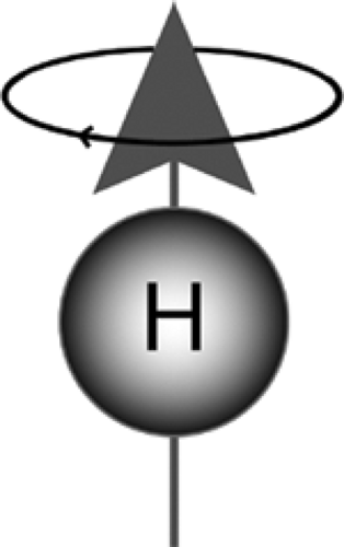 Figure 9-1 The nuclear magnetic moment. Spinning (precessing) anatomic nuclei (“spins”) generate small local magnetic fields analogous to the spinning planets. The magnitude of the magnetic moment depends on the rate of precession, or frequency, of the nucleus. The vector sum of individual magnetic moments for a pool of hydrogen nuclei (“protons”) in fat or water is the essential parameter measured in clinical MRI. (Courtesy of Synarc, Inc.) |
Where γ is the spin’s gyromagnetic ratio, B0 is the strength of the main static magnetic field (for example, 1.5 T), and ω is the proton, or spin resonant frequency in that field. This resonant frequency relationship means that after the spins are tipped into the transverse plane by the B1 pulse, they precess about the longitudinal axis along B0. When the RF (B1) tip-down pulse is turned off, the spins continue to precess. They act as tiny bar magnets, creating their own rotating magnetic field. This changing magnetic field induces a signal across the terminals of the same coil that was used to create the field, because the resonant frequency is the same (Fig. 9-3b). This signal is then used to generate the MR images by computerized Fourier transformation.
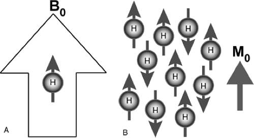 Figure 9-2 Longitudinal magnetization. A, Protons placed within the strong magnetic field B0 (Large open arrow) in the bore of a MRI magnet tend to align their magnetic moments (small arrow) parallel or anti-parallel with this large magnetic field. B, Protons have a slight affinity for parallel alignment, creating a net magnetic moment M0. The magnitude of this net longitudinal magnetic moment and therefore the maximal signal that could be generated during imaging varies directly with the field strength B0 of the MRI magnet. (Courtesy of Synarc, Inc.) |
MR imaging uses three types of coils. The main magnetic field, B0, is created by a superconducting magnet enclosed in a cylindrical cryostat. These magnets must be both strong (field strengths range between 0.2 T and 11 T) and very uniform (within 1 part per million in the imaging volume) in order to precisely set spin frequency. Whole-body scanners are currently limited to a maximum strength of 3 T to 4 T, with most clinical systems ranging from 0.5 T to 3 T. The second coil that creates the RF B1 field is a birdcage-shaped coil that sits permanently within the main B0 coil. Smaller birdcage coils that fit certain volumes, such as the head or extremities, can be placed in the bore as a substitute. Even smaller ring-shaped coils of 10 mm to 100 mm in diameter can be placed directly on the region to be imaged. There is a great advantage in using the smallest possible receive coil, because these coils are not as sensitive to tissues outside the volume of interest, which contribute significantly to image noise. The greatest gain in image Signal-to-noise ratio (SNR) is then achieved by starting with the most appropriate RF coil. The third type of coil used in MR is the gradient coil, of which there is one for each of the three axes. These coils create much smaller magnetic fields that point in the same direction of B0, but vary as a function of distance to the coil. The strength of the linearly varying magnetic fields created by these coils is changed rapidly during an MR exam so that only spins in certain locations have frequencies in the range of those to which the receive coil is sensitive. The gradients force spins to move away from each other in frequency and then return to the same frequency to be in phase. This process is referred to as gradient echo formation. Both higher gradient amplitudes and faster gradient switching rates achieve echoes more quickly and result in shorter scan times.
The two main types of echoes in MR imaging are the gradient echoes (GREs) previously mentioned and spin
echoes (SEs). SEs rephase protons with a 180 degree RF refocusing pulse. This pulse reverses phase position of the spins, flipping the fastest precessing spins behind the slowest precessing ones. After the phase reversal provided by the refocusing pulse, the fastest-moving spins continue at the same precession speeds and catch up so that all spins refocus to a coherent signal. A useful analogy to this process is a track race, halfway through which, the race is reversed so that all runners finish together at the starting line, assuming they maintain constant running speed.
echoes (SEs). SEs rephase protons with a 180 degree RF refocusing pulse. This pulse reverses phase position of the spins, flipping the fastest precessing spins behind the slowest precessing ones. After the phase reversal provided by the refocusing pulse, the fastest-moving spins continue at the same precession speeds and catch up so that all spins refocus to a coherent signal. A useful analogy to this process is a track race, halfway through which, the race is reversed so that all runners finish together at the starting line, assuming they maintain constant running speed.
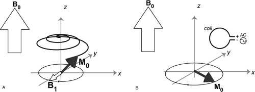 Figure 9-3 RF excitation of transverse magnetization. A, The net proton magnetization M0 that is longitudinally aligned with the high magnetic field B0 (large open arrow) in the MRI magnet bore will realign (resonate) with a second relatively smaller magnetic field B1 (small open arrow) if this new field is tuned to the proton precessional frequency. Since this resonant frequency is in the same range as radio waves, this second field is called a radio-frequency (RF) pulse. B, The RF pulse can be played for a specific duration given the pulse amplitude to produce a full 90° rotation of the net magnetization M0, called the flip angle. This realigned (flipped) magnetic moment (gray vector arrow) will continue to rotate transversely once the RF pulse is turned off to induce an alternating current (by Faraday’s Law) in the wire of the receiver coil placed near the patient. This induced current is the basis for the MR image. (Courtesy of Synarc, Inc.) |
The time it takes for echo formation is called the echo time, or TE. The total time it takes for both an RF excitation and a gradient echo formation/signal acquisition is the repetition time, or TR. TR can be as short as a few milliseconds or as long as a few seconds. The number of repetition times to form an image depends on the imaging method and whether 2D or 3D images are reconstructed. The length of the TR depends on the way the gradients refocus spins after allowing or forcing them to dephase.
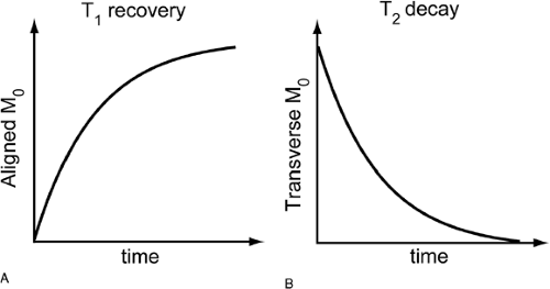 Figure 9-4 T1 T2 relaxation. When the rotating 90° RF pulse is turned off, the transversely oriented magnetic moment re-aligns with the static field of the magnet B0. A, This recovery of longitudinal magnetization is called T1 relaxation, and the parameter, T1, is a measure of the rate of this recovery. If the 90° RF pulse is repeated before longitudinal magnetization has fully recovered, only this smaller longitudinal component is flipped into the transverse plane and the image signal is correspondingly lower—these protons are said to be partially saturated. B, As the longitudinal magnetization re-grows, the transverse component decays. This is called T2 relaxation. (Courtesy of Synarc, Inc.) |
Echoes create the signal for MR images, and TE/TR selection is the mechanism by which contrast is generated between different tissues. As soon as the RF pulse is turned off after excitation, the protons slowly return to their original alignment with the static main field of the magnet (Fig. 9-4). This process of recovering longitudinal magnetization and decaying transverse magnetization is called relaxation. T1 and T2 are the time constants with which this occurs. T1 is the time necessary for the longitudinal magnetization to recover, and T2 is the time for the transverse magnetization to decay. Both of these vary from tissue to tissue, depending
on the microenvironments of the different proton populations. T1 and T2 are therefore tissue characteristics that allow varying MR acquisition timing to generate contrast between tissues. Table 9-1 gives approximate values of different tissues in the knee at a main field strength of 1.5 T.
on the microenvironments of the different proton populations. T1 and T2 are therefore tissue characteristics that allow varying MR acquisition timing to generate contrast between tissues. Table 9-1 gives approximate values of different tissues in the knee at a main field strength of 1.5 T.
TABLE 9-1 APPROXIMATE T1 AND T2 RELAXATION TIMES OF TISSUES IN THE KNEE AT 1.5 T | ||||||||||||||||||||||||
|---|---|---|---|---|---|---|---|---|---|---|---|---|---|---|---|---|---|---|---|---|---|---|---|---|
| ||||||||||||||||||||||||
T1 relaxation, for example, occurs rapidly in fat, while water (abundant in muscle) shows slow T1 relaxation (Fig. 9-5A). T1 also varies slightly with the magnetic field strength so that relaxation of the longitudinal magnetization back to equilibrium is somewhat shorter at lower main field strengths. Under conditions of rapid RF pulsing, slow T1 substances such as water are not given sufficient time to recover between the pulses. Thus, there is little longitudinal magnetization available to be tipped again to create signal, and these substances therefore exhibit low signal intensity. Shorter T1 substances such as fat need less time for longitudinal regrowth and show higher signal intensity (Fig. 9-5A). Short TR sequences therefore generate contrast (relative signal intensity difference) among tissues on the basis of differences in T1 and are accordingly referred to as T1-weighted (Fig. 9-6).
Image contrast is also influenced by T2 relaxation. While the longitudinal magnetization is regrowing after the RF pulse is turned off, the transverse magnetization is slowly decaying. Although not intuitive, the rate of T2 relaxation is not necessarily coupled to the rate of T1 relaxation, other than that the time for T2 relaxation is always shorter than that for T1. Although T1 depends partly on the strength of the main static field, T2 remains constant across all field strengths. As T2 relaxation occurs, the transverse magnetization, and therefore signal, decrease. So, although shorter T1 species are brighter on T1-weighted images, the longer T2 species tissue is brightest on T2-weighted images (Fig. 9-5B). Freely mobile water protons (such as in synovial fluid) show slow T2 relaxation and therefore retain signal over time, whereas constrained or “bound” water protons (such as by collagen or proteoglycan) show rapid T2 relaxation and signal decay (Fig. 9-5B, Fig. 9-6).
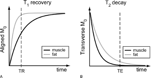 Figure 9-5 Effect of TR/TE on signal intensity. Repetition time (TR) is the time between successive RF pulses in an imaging sequence. Typically, 192 to 256 repetitions are necessary to generate an MR image. If the TR is less than five times the T1 of a substance, there is insufficient time for complete recovery of longitudinal, or aligned magnetization and signal intensity after subsequent excitations is decreased. A, As TR is shortened, tissues with longer T1 relaxation times (e.g., muscle) begin to lose signal first, while tissues with shorter T1 relaxation times (e.g., fat) retain signal until the TR is very short. Short-TR sequences thus generate T1 contrast among tissues and are called T1-weighted. Echo time (TE) is the time between the initiating RF pulse and the point at which spins are refocused either by a 180° rephasing RF pulse (spin-echo) or gradient reversal waveform (gradient-echo). Substances with longer T2 relaxation times (e.g., fat) retain more signal intensity on long-TE(T2-weighted) sequences. B, As TE is lengthened, signal from tissues with shorter and longer T2 relaxation times undergo more decay, changing the contrast. Note that for each value of TE and TR, the contrast between any two tissues is proportional to the difference in signal level, or transverse M0, between the two. In the case of T1-weighted sequences, reductions in the aligned M0 translate into reductions in the transverse M0 after subsequent RF excitations.) (Courtesy of Synarc, Inc.) |
In addition to the effects of neighboring protons on each other (T2 relaxation), heterogeneities in the static magnetic field or off-resonance caused by a chemical shift (as with the 220 Hz difference in fat) cause protons to dephase and lose additional transverse magnetization strength. This is noted as T2‘ relaxation. The combined effects of proton
dephasing and T2 signal loss result in an overall faster decay in transverse magnetization called T2*, which is defined as:
dephasing and T2 signal loss result in an overall faster decay in transverse magnetization called T2*, which is defined as:
| 1 | 1 | 1 | ||
| – | = | – | + | – |
| T2 | T2 | T2 |
Signal lost to fixed magnetic heterogeneity, but not that lost to T2 relaxation, can be recovered using the spin echoes already mentioned.
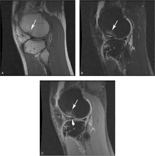 Figure 9-6 T1, T2, and PD-weighted MRI. A, Sagittal T1-weighted spin-echo image of a knee depicts structures that contain fat (short T1) with high signal intensity, and structures that contain water (long T1) with low signal intensity. The small differences in T1 relaxation time among synovial fluid, articular cartilage, and muscle do not generate substantial contrast among these structures on this image. It is difficult, therefore, to delineate the entire articular cartilage surface in this slice. B, T2-weighted fast spin-echo image of the same knee depicts synovial fluid (long T2) with higher signal intensity. Water in articular cartilage and muscle is relatively bound (short T2); these structures therefore show low signal intensity. The dynamic range is much improved with the use of fat suppression, hence the dark marrow in bone. High intrinsic contrast between cartilage and synovial fluid makes this technique useful for delineating the articular surface. C, Proton-density weighted, fat-suppressed fast spin-echo image of the same knee uses a shorter echo time, making cartilage signal brighter. Bone marrow edema is visible in all three images (long arrow) and a small meniscal tear is best visualized in the PD-FSE image (short arrowhead). (Courtesy of Synarc, Inc.) |
Local perturbations of the magnetic field typically arise at interfaces between substances that differ considerably in magnetic susceptibility (the degree to which a substance magnetizes in the presence of a magnetic field), such as between soft tissue and gas, metal, or heavy calcification. Severe T2* at these sites is referred to as magnetic susceptibility effect. Spin-echo refocusing RF pulses correct for fixed magnetic heterogeneities and therefore can provide
images with true T2 contrast. The gradient-echo technique, which relies solely on pre-winding and rewinding gradient waveforms before and after signal acquisition, is faster than spin-echo. However, it does not correct for off-resonance effects and therefore provides only T2*-weighted images. These images are highly vulnerable to magnetic susceptibility effects, such as those caused by metallic prostheses, and can result in large signal voids in the vicinities of metal implants. Note that while SNR increases with higher field strength, artifacts from magnetic susceptibility differences become more severe.
images with true T2 contrast. The gradient-echo technique, which relies solely on pre-winding and rewinding gradient waveforms before and after signal acquisition, is faster than spin-echo. However, it does not correct for off-resonance effects and therefore provides only T2*-weighted images. These images are highly vulnerable to magnetic susceptibility effects, such as those caused by metallic prostheses, and can result in large signal voids in the vicinities of metal implants. Note that while SNR increases with higher field strength, artifacts from magnetic susceptibility differences become more severe.
Finally, diffusion of protons (for example, water) within a specimen during the acquisition of an MR image results in loss of phase coherence among the protons and therefore a loss in signal. This effect is usually insignificant in conventional MRI but can be augmented with the use of strong magnetic field gradients such as those employed in MR microimaging. Water diffusivity is thus an additional tissue parameter measurable with MRI.6,7
Both T1-weighting (short TR) and T2-weighting (long TE) involve discarding MR signal. If these effects are eliminated, signal intensity reflects only the proton density. Accordingly, long-TR/ short-TE images are often referred to as proton density-weighted. However, even the shortest finite TE attainable is too long to completely escape T2 relaxation, and extremely long TRs (> 2500 ms) are not practical for imaging in vivo. Therefore, even so-called proton density-weighted images contain some T1 and T2 contrast (Fig. 9-6, Fig. 9-14).
Another consequence of the relaxation that occurs from TR to TR is that during the first few repetitions, the signal will be different strengths. Because the magnetization has not fully recovered after the first TR, the second signal acquisition has less available signal to be tipped into the transverse plane. The third acquisition will differ from the second, and so forth. Eventually, however, these differences from TR to TR become smaller and smaller, and the signal is said to be in the steady state. The effort to shorten this transient time to maximize useful imaging time, as well as methods of manipulating spins at the end of each TR to reach this condition more quickly, has been an active area of imaging research.8,9,10.
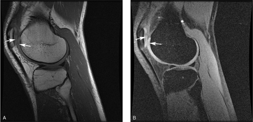 Figure 9-7 Augmenting T1 contrast with fat suppression. A, Sagittal, T1-weighted spin-echo image of a knee acquired with a TR of 500 ms, at the short end of the usual range (500 ms to 700 ms) depicts the articular cartilage (arrows) with a slightly higher signal intensity than the adjacent synovial fluid. Contrast between cartilage and water is greater on this shorter-TR image than on the conventional T1-weighted image shown in Fig. 9-6A (TR = 600 ms), but is still overshadowed by the greater T1 contrast between fat and other tissues in the image. B, The same sequence repeated with fat suppression generates greater contrast between articular cartilage (arrows) and synovial fluid as their pixel intensities are rescaled across a broader range of gray scale values. The same effect can be achieved with water-selective excitation. (Courtesy of Synarc, Inc.) |
Subtle T1 contrast (for example, between articular cartilage and synovial fluid) is usually overshadowed on T1-weighted images by the far greater difference in signal intensity that exists between fat and most other tissues, because the presence of fat increases the dynamic range of the resulting images. However, by selectively suppressing the signal intensity of fat, it is possible to expand the scale of image intensities across smaller differences in T1 and thus to augment residual T1 contrast (Fig. 9-7). Another application of fat suppression is to increase contrast between fat and other substances, such as methemoglobin and gadolinium (Gd)-containing contrast material, which also show rapid T1 relaxation. The most widely used technique for fat suppression is based on the chemical shift phenomenon: Because the frequency of protons in fat differs from that of protons in water, the magnetization of fat
(or water) can be selectively suppressed by a specifically tuned RF pulse at the beginning of the sequence (Fig. 9-8). This RF pulse, which is centered on the fat frequency instead of the water frequency, prematurely tips down the fat spins so that when the sequence RF tip-down pulse is played out, there is no longitudinal magnetization in fat available to produce a signal.
(or water) can be selectively suppressed by a specifically tuned RF pulse at the beginning of the sequence (Fig. 9-8). This RF pulse, which is centered on the fat frequency instead of the water frequency, prematurely tips down the fat spins so that when the sequence RF tip-down pulse is played out, there is no longitudinal magnetization in fat available to produce a signal.
A similar technique can also be used to suppress the signal of water indirectly, through a mechanism called magnetization transfer. In this case, direct suppression of tightly constrained protons in macromolecules such as collagen, which are thermodynamically coupled to freely mobile protons in bulk water, evokes a transfer of magnetization from the water proton pool to the macromolecular pool to maintain equilibrium. This manifests as a loss of longitudinal magnetization and therefore signal intensity from water—in proportion to the relative concentrations of the two proton pools in the tissue and the specific rate constant for the equilibrium reaction. Because collagen (unlike fat) is strongly coupled to water in this way, cartilage and muscle exhibit pronounced magnetization-transfer effects.11,12,13,14
Magnetization-transfer techniques are therefore useful for imaging the articular cartilage and could potentially be used to quantify the collagen content of this tissue.
The two most important parameters for describing the extent of tissue coverage are image resolution and field of view (FOV). Both of these parameters depend on the strength of the gradients, on gradient switching speed, and on how the gradient waveforms are played out during the acquisition. Finer resolution requires an increase in the number of frequencies that must be sampled and therefore longer gradient waveforms. Images that have larger FOV (that is, are zoomed out to show more anatomy) require frequencies to be more precisely resolved, which means that gradient waveforms must be lower in amplitude and of longer time duration. So, both resolution and FOV are also dependent on the amount of time available within a single TR to keep scan times reasonable, patient motion reduced, and contrast/signal available despite relaxation effects.
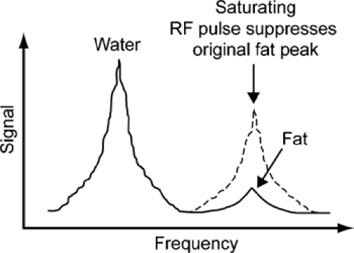 Figure 9-8 Frequency-selective fat suppression. The chemical-shift phenomenon separates the resonant frequencies of water and fat (by 220 Hz at a magnetic field strength of 1.5 T). This allows the longitudinal magnetization of either of these proton pools to be selectively suppressed by an RF pulse tuned to the correct resonant frequency. Since the resonant frequency and the magnitude of the chemical shift both depend on magnetic field strength, this method of fat suppression is dependent on the homogeneity of the static magnetic field and is not feasible at very low field strengths. |
In 2D imaging, a slice is selected during excitation, and the other two spatial axes are localized down and across the image plane during acquisition. Alternatively, 3D data sets can be acquired by exciting all spins and playing localizer gradients on all three axes during acquisition. In either of these cases, dimensions of the individual volume elements, or voxels, comprising it define the spatial resolution of an MR image. Voxel size is determined by multiplying the slice thickness by the size of the in-plane subdivisions of the image, the pixels (picture elements). Pixel size, in turn, is determined by dividing the FOV by the image matrix, which most commonly ranges between 256 × 128 and 256 × 256 for knee imaging. The key point of pixel size is the smaller the pixel, the finer the spatial resolution. Typical sizes for FOV in knee imaging are around 14 cm.
All signals within a single voxel are averaged. Therefore, if an interface with high signal intensity on one side and low signal intensity on the other side passes through the middle of a voxel, then the interface is depicted as an intermediate signal intensity band the width of the voxel (Fig. 9-9). This effect is known as partial-volume signal averaging. However, as voxel size decreases, so does SNR. Accordingly, high-resolution imaging requires sufficient SNR to support the spatial resolution. SNR can be increased by shortening TE (less T2 decay), increasing TR (more T1 recovery), imaging at higher field strength (greater longitudinal magnetization), or utilizing specialized coils that reduce noise (small surface coils, quadrature coils, or phased arrays of small coils).15,16 Specialized sequences, such as those that fully refocus spin dephasing from T2* effects, also provide greater SNR.
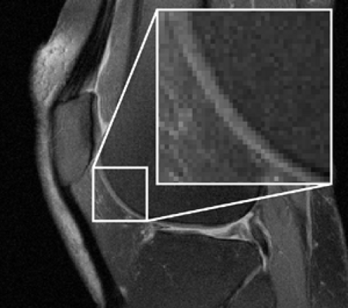 Figure 9-9 Partial volume averaging. The smallest element of an MR image is the individual voxel (pixel size • slice thickness). Different signal intensities within a single voxel are averaged. This effect is most noticeable at high contrast interfaces as shown in the magnified view of the femoral cartilage on this sagittal, fat-suppressed, T1-weighted gradient-echo image of a knee. (Courtesy of Synarc, Inc.) |
Imaging Articular Cartilage
Magnetic Resonance Imaging Appearance of Articular Cartilage: Contrast Mechanisms
The signal behavior of articular cartilage on MRI reflects the complex biochemistry and histology of this tissue. The high water content (proton density) of articular cartilage forms the basis for MR signal. Water content in this tissue depends on the delicate balance between the swelling pressure of the aggregated proteoglycans and the counter resistance of the fibrous collagen matrix. But, in general terms, changes in cartilage proton density tend to be relatively small (typically <20%). Because the water constitutes approximately 70% of the weight of normal articular cartilage, proton density itself offers little scope for generating image contrast between cartilage and adjacent synovial fluid. However, this fundamental MRI signal in cartilage is modulated by a number of processes, including T1 relaxation, T2 relaxation, magnetization transfer, water diffusion, magnetic susceptibility, and interactions with contrast agents. These processes provide many different mechanisms for delineating cartilage morphology and probing its composition.
For comparison, Table 9-1 gives the T1 and T2 values of tissues in the knee. The T1 of articular cartilage at 1.5 T is approximately 800 ms. This time is much shorter than the T1 of adjacent synovial fluid, (2500 ms) but still longer than the T1 of subarticular marrow fat (260 ms). The gray scale on a conventional T1-weighted SE image is then so dominated by fat that the contrast between articular cartilage and adjacent synovial fluid is normally difficult to appreciate (Fig. 9-6). Intrinsic T1-contrast can be augmented slightly by shortening TR, but a more powerful approach is to suppress the fat signal or selectively excite protons in water, and rescale the smaller residual T1 contrast across the image. This generates images in which articular cartilage is depicted as an isolated high signal intensity band in sharp contrast with adjacent low signal intensity joint fluid, and nulled fat in adipose tissue (for example, Hoffa’s fat pad) and bone.12,17 Fat suppression also eliminates chemical-shift artifacts that distort the cartilage—bone interface and complicate dimensional measurements.
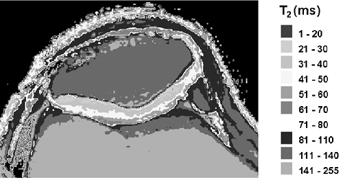 Figure 9-10 T2 Relaxation of normal adult articular cartilage. T2 map generated from multislice, multi-echo (11 echoes: TE = 9, 18, … 99 ms) spin-echo images acquired at 3 T shows increasing T2 toward the articular surface. (Courtesy of B. J. Dardzinski, Ph.D. University of Cincinnati College of Medicine.) |
T2 relaxation is another tissue characteristic that can be harnessed to image the articular cartilage. Fibrillar collagen in the articular cartilage immobilizes tissue water protons and promotes dipole-dipole interactions among them, increasing T2 relaxation and therefore signal decay. The T2 of normal articular cartilage increases from approximately 30 ms in the deep radial zone to 70 ms in the transitional zone18 (Fig. 9-10). Above the transitional zone, the superficial tangential zone shows extremely rapid T2 relaxation because of its densely matted collagen fibers. This radial heterogeneity of T2 gives articular cartilage a laminar appearance on all but extremely short-TE images.19 The pattern of T2 variation can be explained, to some extent, by the heterogeneous distribution of collagen in this tissue, but is also affected by the orientation of collagen fibrils relative to the static magnetic field (B0). T2 anisotropy in cartilage manifests as decreased signal decay in regions where the collagen fibrils are oriented at 55° to B0.19,20,21,22 This so-called “magic-angle” phenomenon is responsible for areas of mildly elevated signal intensity in the radial zone of appropriately oriented cartilage segments on intermediate-TE images (Fig. 9-11). It is also one explanation for the slower T2 seen in the transitional zone. Collagen fibrils in this zone are slightly sparser than in the radial zone, but more importantly they are also highly disorganized. Accordingly, a significant proportion of the fibrils in the transitional zone are angled at 55° to B0regardless of the orientation of the knee in the magnet. With sufficiently long TE (<80 ms), normal articular cartilage appears diffusely low in signal intensity even in regions normally affected by this magic-angle phenomenon.
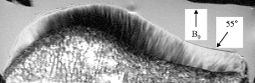 Figure 9-11 Magic-angle phenomenon in articular cartilage. High-resolution spin-echo image of the patellar cartilage shows low signal intensity due to T2 relaxation in the radial zone of the central portion of the cartilage, where collagen is aligned with the static magnetic field (B0.) Increased signal intensity (arrow) indicative of prolonged T2 can be seen in areas where the collagen is oriented at approximately 55° relative to B0. (Courtesy of D. Goodwin, and J. Dunn, Dartmouth Medical School.) |
Superimposed upon these histological and biochemical causes of laminar appearance in articular cartilage are patterns created by truncation artifacts.23,24 This manifests as one or several thin horizontal bands of low signal intensity midway through the cartilage on short-TE images. Truncation artifacts are less common on high-resolution images, but usually present on fat-suppressed 3D spoiled gradient-recalled (SPGR) images generated with most clinical protocols.
Long-TE images provide high contrast between articular cartilage and adjacent synovial fluid, but poor contrast between cartilage and bone. Shorter-TE images improve
cartilage bone contrast, but are vulnerable to magic-angle effects. Fast SE (FSE) combines T2 effects with magnetization transfer to decrease signal intensity in articular cartilage.25,26 Signal loss due to magnetization transfer results from equilibration of longitudinal magnetization between nonsaturated freely mobile protons in water and saturated restricted protons in macromolecules, such as collagen, that have been excited off the resonant frequency of free water during multi-slice imaging.11,12,14,25,26,27 The effect is exaggerated with FSE imaging because of the multiple 180° RF pulses used with this technique. Accordingly, intermediate TE (∼40 ms) FSE images show relatively low signal intensity in articular cartilage while preserving high signal intensity in synovial fluid and subjacent bone marrow to delineate the articular cartilage with high contrast (Fig. 9-13). Both intermediate and long TE FSE images offer relatively good morphological delineation of articular cartilage in less time than is required for high-resolution fat-suppressed 3D-GRE images. The choice of which TE to use depends on the objectives of the imaging and how they relate to the range of normal and pathological T2 heterogeneity found in articular cartilage.
cartilage bone contrast, but are vulnerable to magic-angle effects. Fast SE (FSE) combines T2 effects with magnetization transfer to decrease signal intensity in articular cartilage.25,26 Signal loss due to magnetization transfer results from equilibration of longitudinal magnetization between nonsaturated freely mobile protons in water and saturated restricted protons in macromolecules, such as collagen, that have been excited off the resonant frequency of free water during multi-slice imaging.11,12,14,25,26,27 The effect is exaggerated with FSE imaging because of the multiple 180° RF pulses used with this technique. Accordingly, intermediate TE (∼40 ms) FSE images show relatively low signal intensity in articular cartilage while preserving high signal intensity in synovial fluid and subjacent bone marrow to delineate the articular cartilage with high contrast (Fig. 9-13). Both intermediate and long TE FSE images offer relatively good morphological delineation of articular cartilage in less time than is required for high-resolution fat-suppressed 3D-GRE images. The choice of which TE to use depends on the objectives of the imaging and how they relate to the range of normal and pathological T2 heterogeneity found in articular cartilage.
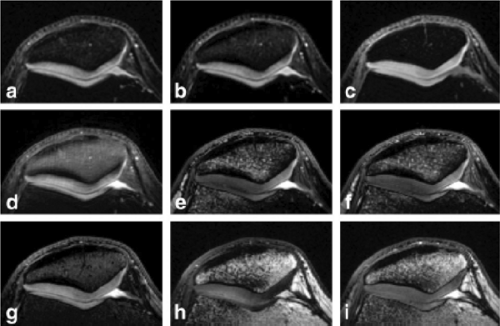 Figure 9-12 Comparison of FSE and SPGR to DEFT and three variants of SSFP. Axial patellofemoral water images from a normal volunteer using A, FSE (TR = 1800 ms), B, FSE (TR = 3200 ms), C, SPGR, D, DEFT, E, LC-SSFP, F, FEMR, and G, FS-SSFP. Fat images using LC-SSFP H, and FEMR I, require no additional scan time. Water images from DEFT D, and the SSFP-based techniques (e.g., FS-SSFP, LC-SSFP, and FEMR) all demonstrate both bright cartilage and excellent contrast with synovial fluid. ( Hargreaves, B.A., Gold, G.E., Beaulieu, C.F., et al. Comparison of new sequences for high-resolution cartilage imaging. Magn Reson Med 49:700–709, 2003. ) |
Magnetic Resonance Pulse Sequences for Imaging Articular Cartilage Morphology
Two pulse sequences are the clinical workhorses of knee imaging: T1-weighted spoiled GRE, referred to as SPGR or FLASH (fast low-angle shot) and T2-weighted fast spin-echo (FSE), or turbo spin-echo (TSE). SPGR provides 3D acquisition in reasonable scan times and is currently the most available clinical option for quantitative measurements of cartilage volume.28 However, it does not provide strong cartilage-synovial fluid contrast and is susceptible to T2* dephasing. FSE is much more robust to off-resonance, and its contrast is not weighted by T2* However, the method requires a longer repetition interval, and therefore scan times for 3D acquisition would be prohibitively long.
Fat-suppressed, T1-weighted 3D SPGR is easy to use and widely available, and has become a popular MRI technique for delineating articular cartilage morphology.12,17,29,30,31,32 However, the sequence provides poor cartilage-synovial fluid contrast, making depiction of cartilage surface defects difficult. Driven equilibrium (DE, DEFT, or FR [Fast Recovery] as in FR-SE) produces higher cartilage-synovial fluid contrast than either FSE or SPGR (Fig. 9-12), making it a good choice for imaging cartilage surface defects. The contrast is based on tissue T2/T1, which makes synovial fluid brighter. Although DEFT provides shorter scan times and allows for 3D imaging, other sequences with higher SNR efficiency are better choices for cartilage volume measurement.
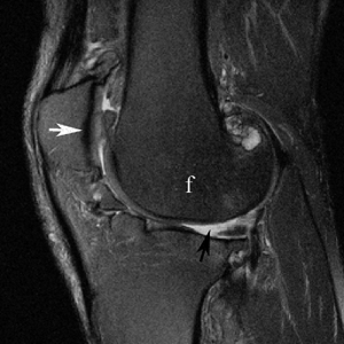 Figure 9-13 Fast spin echo imaging of cartilage. Sagittal T2-weighted fast spin echo image of the knee shows high contrast between the low signal intensity articular cartilage (white arrow) and adjacent high signal intensity synovial fluid (black arrow) and intermediate signal intensity subchondral marrow fat (f). (Courtesy of Synarc, Inc.)
Related posts:Stay updated, free articles. Join our Telegram channel
Full access? Get Clinical Tree
 Get Clinical Tree app for offline access

|


